Astro.IQ
Using Ballistic Guesses
In the process of trajectory optimisation, often the most severe bottleneck in performance manifests in supplying an initial guess. One of the simplest ways to supply an initial guess is to initialise the nonlinear programme decision vector randomly within the state and control space, and respectively. At first this may seem like a sufficient idea; however, if one brings their attention to the problem’s dynamic constraints, this will certainly be ineffective.
Examining a two dimensional planetary lander, whose dynamics are governed by the first order system ordinary differential equations
, it is quite unsurprising that a random distribution of state nodes is likely to prevent the optimiser from converging to a feasible solutions. A smarter way to provide a guess that looks more natural, with respect to the system’s dynamics, is to provide a ballistic guess, otherwise known as an uncontrolled trajectory.
To do this one simply propagates or numerically integrates the system’s dynamics from an initial state to an arbitrary final time , and then samples evenly distributed nodes along the trajectory to subsequently input to the optimiser. However, one must ensure that all these nodes of the system’s state are within the problem’s state space bounds, that is .
Astro.IQ Implementation
Within the Astro.IQ framework, one can easily
- Define their own dynamical model
- Choose an optimisation method
- Optimise the trajectory with any PyGMO algorithm.
One first imports the necessary resources
from Trajectory   import Point_Lander
from Optimisation import Trapezoidal
then instantiates the dynamical model.
# Instantiate a dynamical model and look at details
Model = Point_Lander()
Optimisation Transcription
The problem is then transcribed with a chosen optimisation method. In this case the trapezoidal transcription method is used, where the decision vector is
, where the system’s state is given by
and the control by
. In this transcription, the dynamic constraints are enforced by equality constraints given by the trapezoidal quadrature
, where is the number of segments the trajectory is divided into.
# Create a trajectory optimisation problem and look at details
Problem = Trapezoidal(Model, nsegs=50)
Taking a Guess
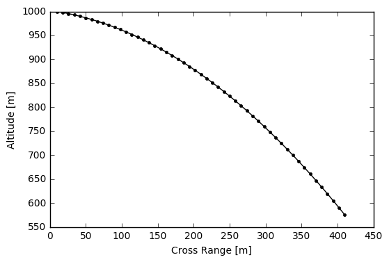
One can show what a ballistic trajectory with a flight time looks like, where the problem’s number of nodes is implicitly passed to the guessing method:
# Guess from a ballistic (uncontrolled) trajectory
tf, state, control = Problem.Guess.Ballistic(tf=20, nlp=False)
# Visualise the guess
import matplotlib.pyplot as plt
plt.plot(state[:,0], state[:,1], 'k.-') # Trajectory
plt.ylabel('Altitude [m]'); plt.xlabel('Cross Range [m]')
plt.show()
Optimising the Trajectory
The optimiser is imported
# Import PyGMO for optimisation
from PyGMO import *
wherein the method of sequential least squares quadratic programming is used:
# Use sequential least squares quadratic programming
algo = algorithm.scipy_slsqp(max_iter=3000, screen_output=True)
A space for any number of decision vectors is allotted:
# Create an empty population space for individuals (decision vectors) to inhabit
pop = population(Problem)
A ballistic decision vector is generated
# Provide a ballistic (uncontrolled) trajectory as an initial guess
zguess = Problem.Guess.Ballistic(tf=20)
, and subsequently added as a chromosome to the space.
# Add the guess to the population
pop.push_back(zguess)
The decision vector is then evolved through the gradient based optimiser until an error tolerance is satisfied, both with respect to the boundary conditions (i.e. arriving at the target state) and dynamic constraints (i.e. abiding to the equations of motions).
# Evolve the individual with SLSQP
pop = algo.evolve(pop)
  NIT    FC           OBJFUN            GNORM
    1   411    -9.500000E+03     1.000000E+00
    2   832    -9.500000E+03     1.000000E+00
    3  1250    -9.500000E+03     1.000000E+00
    4  1671    -9.500000E+03     1.000000E+00
    ⋮   ⋮           ⋮                ⋮
  627 257760    -9.242340E+03     1.000000E+00
  628 258175    -9.242340E+03     1.000000E+00
  629 258590    -9.242340E+03     1.000000E+00
  630 259005    -9.242340E+03     1.000000E+00
Optimization terminated successfully.    (Exit mode 0)
            Current function value: -9242.33995699
            Iterations: 630
            Function evaluations: 259006
            Gradient evaluations: 629
The optimised decision vector is then decoded into the total flight time , the state trajectory , and the sequence of controls .
tf, s, c = Problem.Decode(pop.champion.x)
Trajectory Evaluation
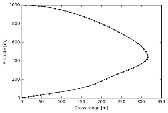
Examining the plot of the optimised position trajectory, the optimisation process seems to have been quite effective.
# x vs. y
plt.plot(s[:,0], s[:,1], 'k.-'); plt.xlabel('Cross range [m]'); plt.ylabel('Altitude [m]')
plt.show()
Control
From optimal control theory, one can analyse how the nature of the system’s control should behave. There is a vector of non physical costate variables
, from which the system’s Hamiltonian is defined
, where the system’s Lagrangian or cost functional is defined as
. From Pontryagin’s maximum principle, one notes that the Hamiltonian must be maximized over the set of all possible controls
, and hence the optimal throttle policy is found as
, where the switching function is
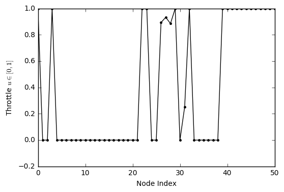
. Hence this describes what is known as bang-bang control, which is characteristic of mass-optimal control policies, where the throttle is either on or off. Plotting the lander’s throttle sequence, it can be seen that this behaviour is emulated, with the exception of a few intermediate values due to the problem’s discretisation.
# Controls (note the bang-off-bang profile indicative of mass optimal control)
plt.plot(c[:,0], 'k.-')
plt.ylabel('Throttle $u \in [0,1]$')
plt.xlabel('Node Index')
plt.show()
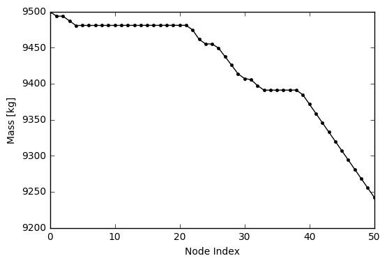
One can also see the lander’s fuel expenditure along its trajecory:
# Plot the propellent usage
plt.plot(s[:,4],'k.-')
plt.ylabel('Mass [kg]')
plt.xlabel('Node Index')
plt.show()
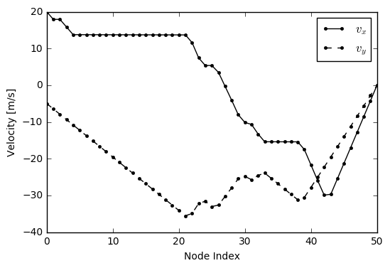
Soft Landing?
The lander not only met its target position, but it also landed softly, meeting its target velocity as desired.
# Soft landing
plt.plot(s[:,2], 'k.-')
plt.plot(s[:,3], 'k.--')
plt.legend(['$v_x$', '$v_y$'])
plt.xlabel('Node Index')
plt.ylabel('Velocity [m/s]')
plt.show()
Want to learn more?
Have a look at the following resources:
- Astro.IQ - for the source code of this software
- Full IPython notebook - for how I did this example
- Practical Methods for Optimal Control Using Nonlinear Programming - to learn about optimal control methods
- Python Parallel Global Multiobjective Optimizer (PyGMO) - to learn about the optimisation platform used