# We first import the resources
import sys
sys.path.append('..')
from Trajectory import Point_Lander
from Optimisation import Hermite_Simpson
from PyGMO import *
from numpy import *
from pandas import *
import matplotlib.pyplot as plt

# We instantiate the problem
prob = Hermite_Simpson(Point_Lander(si=[0,1000,20,-5,9900]))

# Let us first supply a ballistic trajectory as a guess
zguess = prob.Guess.Ballistic(tf=28)

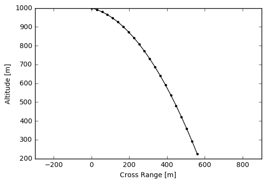
# Decode the guess so we can visualise
tf, cb, s, c = prob.Decode(zguess)

plt.plot(s[:,0], s[:,1], 'k.-')
plt.axes().set_aspect('equal', 'datalim')
plt.xlabel('Cross Range [m]')
plt.ylabel('Altitude [m]')
plt.show()

# Use SLSQP and alternatively Monotonic Basin Hopping
alg1 = algorithm.scipy_slsqp(max_iter=3000, screen_output=True)
alg2 = algorithm.mbh(alg1, screen_output=True)

# Instantiate a population with 1 individual
pop = population(prob)
# and add the guess
pop.push_back(zguess)

# We then optimise the trajectory
pop = alg1.evolve(pop)

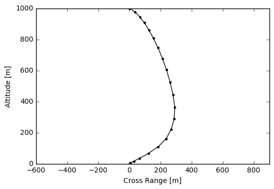
# We now visualise the optimised trajectory
tf, cb, s, c = prob.Decode(pop.champion.x)
plt.plot(s[:,0], s[:,1], 'k.-')
plt.axes().set_aspect('equal', 'datalim')
plt.xlabel('Cross Range [m]')
plt.ylabel('Altitude [m]')
plt.show()

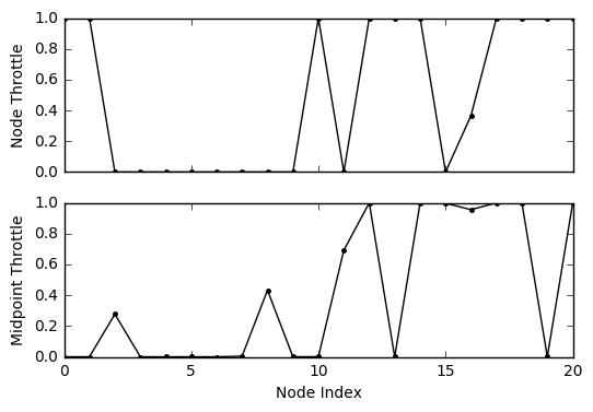
# and look at the control throttle
plt.close('all')
f, ax = plt.subplots(2, sharex=True)
ax[0].plot(c[:,0], 'k.-')
ax[1].plot(cb[:,0], 'k.-')
plt.xlabel('Node Index')
ax[0].set_ylabel('Node Throttle')
ax[1].set_ylabel('Midpoint Throttle')
plt.show()

# We save the optimised trajectory decision vector
save('HSD0', pop.champion.x)

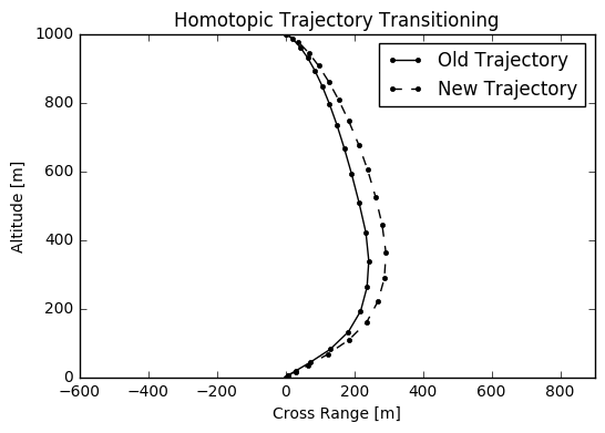
# We perturb the initial state and find a optimsal trajectory
# Decreasing the velocity by a few m/s for demonstration
prob = Hermite_Simpson(Point_Lander(si=[0,1000,10,-5,9900]))
# and create a population for the new problem
pop = population(prob)
# and add the previous population decision vector
pop.push_back(z)

# We then optimise the trajectory, this now will not take long!
pop = alg1.evolve(pop)

# We now compare this new perturbed trajectory to the previous
tf1, cb1, s1, c1 = prob.Decode(pop.champion.x)
plt.close('all')
plt.figure()
plt.plot(s1[:,0], s1[:,1], 'k.-') # The new trajectory
plt.plot(s[:,0], s[:,1], 'k.--') # The old trajectory
plt.legend(['Old Trajectory', 'New Trajectory'])
plt.title('Homotopic Trajectory Transitioning')
plt.axes().set_aspect('equal', 'datalim')
plt.xlabel('Cross Range [m]')
plt.ylabel('Altitude [m]')
plt.show()

# In essence, we will incrementally perturb the dynamical system's
# initial state and repeatedly compute new optimal trajectories.
# So, again we store the new trajectory decisions vector
save('HSD1', pop.champion.x)

# Store the current decision
z = pop.champion.x

# Now we try perturbing the initial position rather
# We instantiate the problem
prob = Hermite_Simpson(Point_Lander(si=[-10,1000,10,-5,9900]))
# and create a population for the new problem
pop = population(prob)
# and add the previous population decision vector
pop.push_back(z)

# We then optimise the trajectory, this now will not take long!
pop = alg1.evolve(pop)

# We now compare this new perturbed trajectory to the previous
tf2, cb2, s2, c2 = prob.Decode(pop.champion.x)

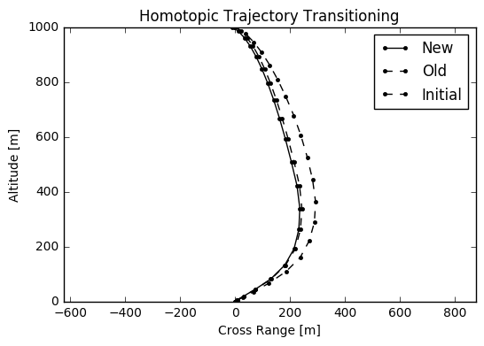
plt.close('all')
plt.figure()
plt.plot(s2[:,0], s2[:,1], 'k.-') # The new trajectory
plt.plot(s1[:,0], s1[:,1], 'k.--') # The old trajectory
plt.plot(s[:,0], s[:,1], 'k.--') # The initial trajectory
plt.legend(['New', 'Old', 'Initial'])
plt.title('Homotopic Trajectory Transitioning')
plt.axes().set_aspect('equal', 'datalim')
plt.xlabel('Cross Range [m]')
plt.ylabel('Altitude [m]')
plt.show()

# Again, save the decision
save('HSD2', pop.champion.x)
z = pop.champion.x

# We instantiate the problem one last time
prob = Hermite_Simpson(Point_Lander(si=[-10,1000,0,-5,9900]))
# and create a population for the new problem
pop = population(prob)
# and add the previous population decision vector
pop.push_back(z)

# We then optimise the trajectory, this now will not take long!
pop = alg1.evolve(pop)

# We now compare this new perturbed trajectory to the previous
tf3, cb3, s3, c3 = prob.Decode(pop.champion.x)

%matplotlib inline
%config InlineBackend.figure_format = 'svg'
plt.close('all')
plt.figure()
plt.plot(s3[:,0], s2[:,1], 'k.-')
plt.plot(s2[:,0], s2[:,1], 'k.--') # The new trajectory
plt.plot(s1[:,0], s1[:,1], 'k.--') # The old trajectory
plt.plot(s[:,0], s[:,1], 'k.--') # The initial trajectory
plt.legend(['New', 'Old'])
plt.title('Homotopic Trajectory Transitioning')
plt.axes().set_aspect('equal', 'datalim')
plt.xlabel('Cross Range [m]')
plt.ylabel('Altitude [m]')
#plt.savefig('Homotopic_Transitioning.pdf', format='pdf',
#           transparent=True, bbox_inches='tight')
plt.show()

# I think we get it now... time to do this more programmatically
# but first we again save the decision vector
z = pop.champion.x
save('HSD3', z)