Training and Using Neuro-Controllers

Data Generation

In order to arrive at the final objective of being able to implement a neuro-controller to optimally control a user specified dynamical system, under this methodology a large database of optimal control trajectories must first be generated. The topological continuation of a system’s dynamics may be exploited to enable rapid generation of many optimal control trajectories, in a what is formally known as homotopy, relating two continuous functions from topological space to another.

Homotopy

As optimising trajectories of complicated nonlinear systems is rather computationally arduous, the topological continuation of a system’s dynamics is exploited in order to render each individual optimisation process expedient. If one generates an optimal trajectory from a particular initial state and then uses the resulting solution to optimise a trajectory from a similar initial state, it would be seen that the optimiser converges incredibly quickly and that the solution is very similar.

Random Walks

In practice, in order to exploit the topological continuation of the system’s dynamics, random walks are performed within user specified boundaries of a dynamical system’s possible initial states, silb, siub. The random walks are done with a step size with respect to a percentage of each state element’s boundary region size.

def Random_Initial_States(model, mxstep=10., nstates=5000.):
    # The model's initial state boundaries
    silb    = model.silb
    siub    = model.siub
    # The size of the boundary space
    sispace = siub - silb
    # Convert the percent input to number
    mxstep  = mxstep*1e-2*sispace
    # Make array
    states = zeros((nstates, model.sdim))
    # First state in between everything
    states[0] = silb + 0.5*sispace
    for i in arange(1, nstates):
        perturb   = random.randn(model.sdim)*mxstep
        # Reverse and decrease the steps of violating elements
        states[i] = states[i-1] + perturb
        badj = states[i] < silb
        states[i, badj] = states[i-1, badj] - 0.005*perturb[badj]
        badj = states[i] > siub
        states[i, badj] = states[i-1, badj] - 0.005*perturb[badj]
    return states

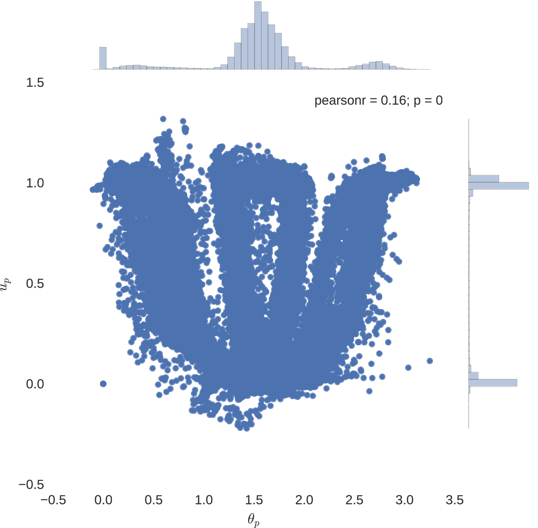
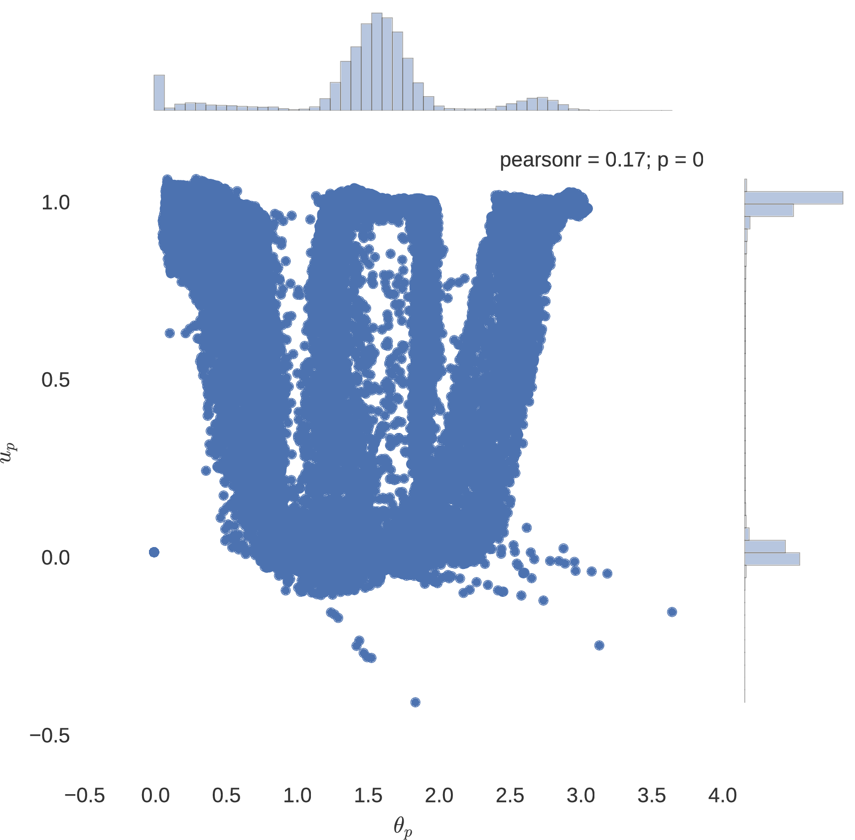
The random walks of initial states, within the position and velocity boundaries of a lander, are shown below.

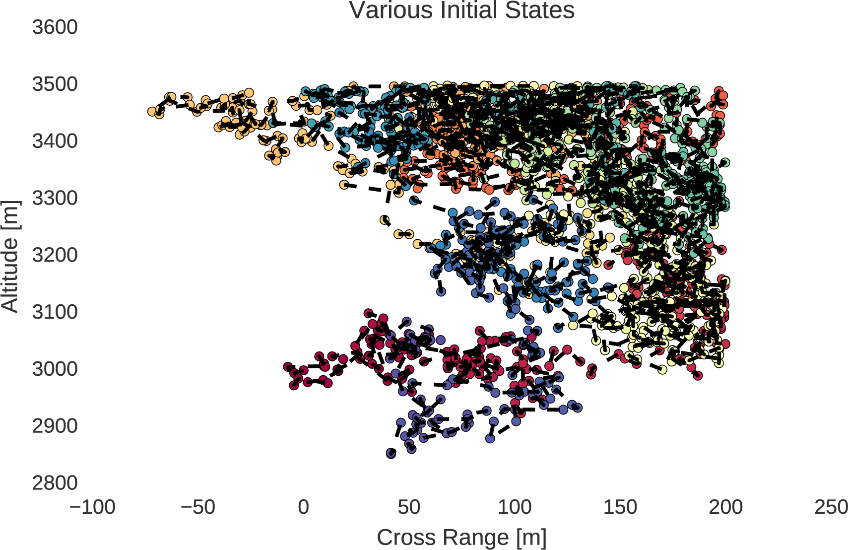
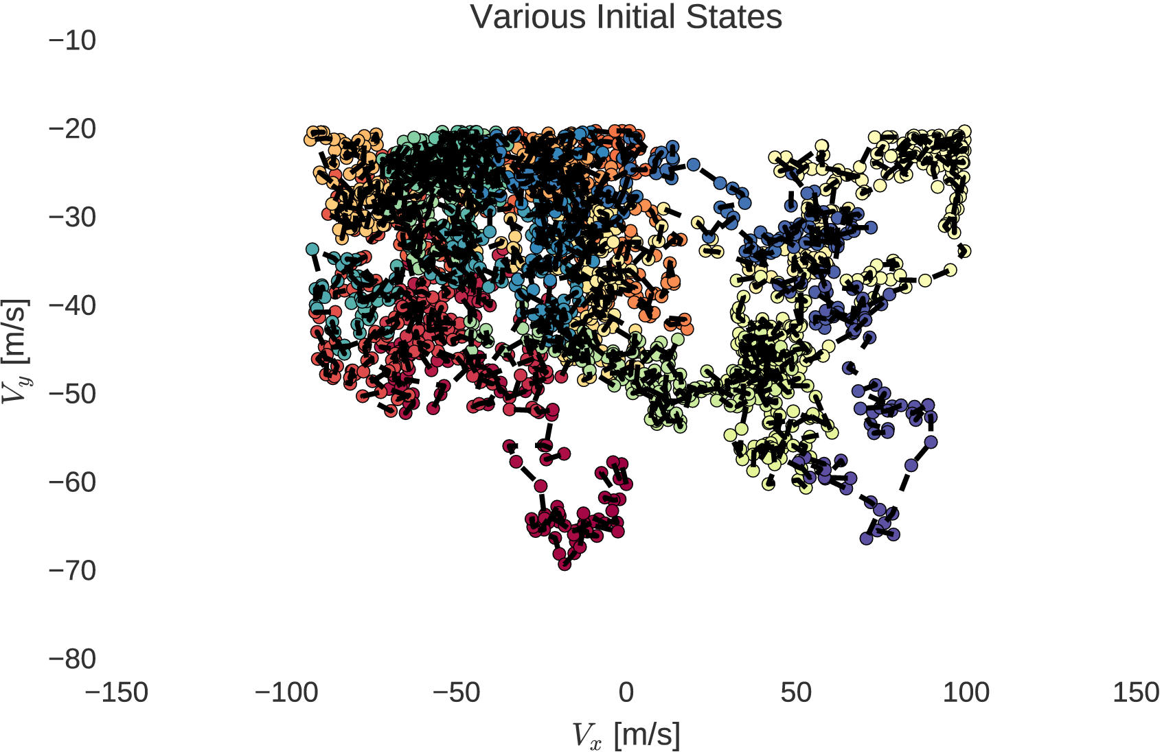
From the generated sequence of initial states, generated in order of similarity through the random walk within bounds, the methods of trajectory optimisation may be employed from each initial state. The optimisation process quickly converges from each subsequent initial state due to their similarities as explained by homotopy. Through this process, a very large database of optimal trajectories can be generated from various initial states.

Case Study: Martian Lander with Atmospheric Effects

Now consider for example a planetary lander encountering the Martian atmosphere

where the system’s control is characterised by $u \in [0,1]$ and $\theta \in [0, \pi]$, the thrust throttle level and direction respectively, and the thrust direction $\theta$ is restricted to only point upward, as would be expected from a landing trajectory optimisation solution. The system’s set of constant parameters are outlined as

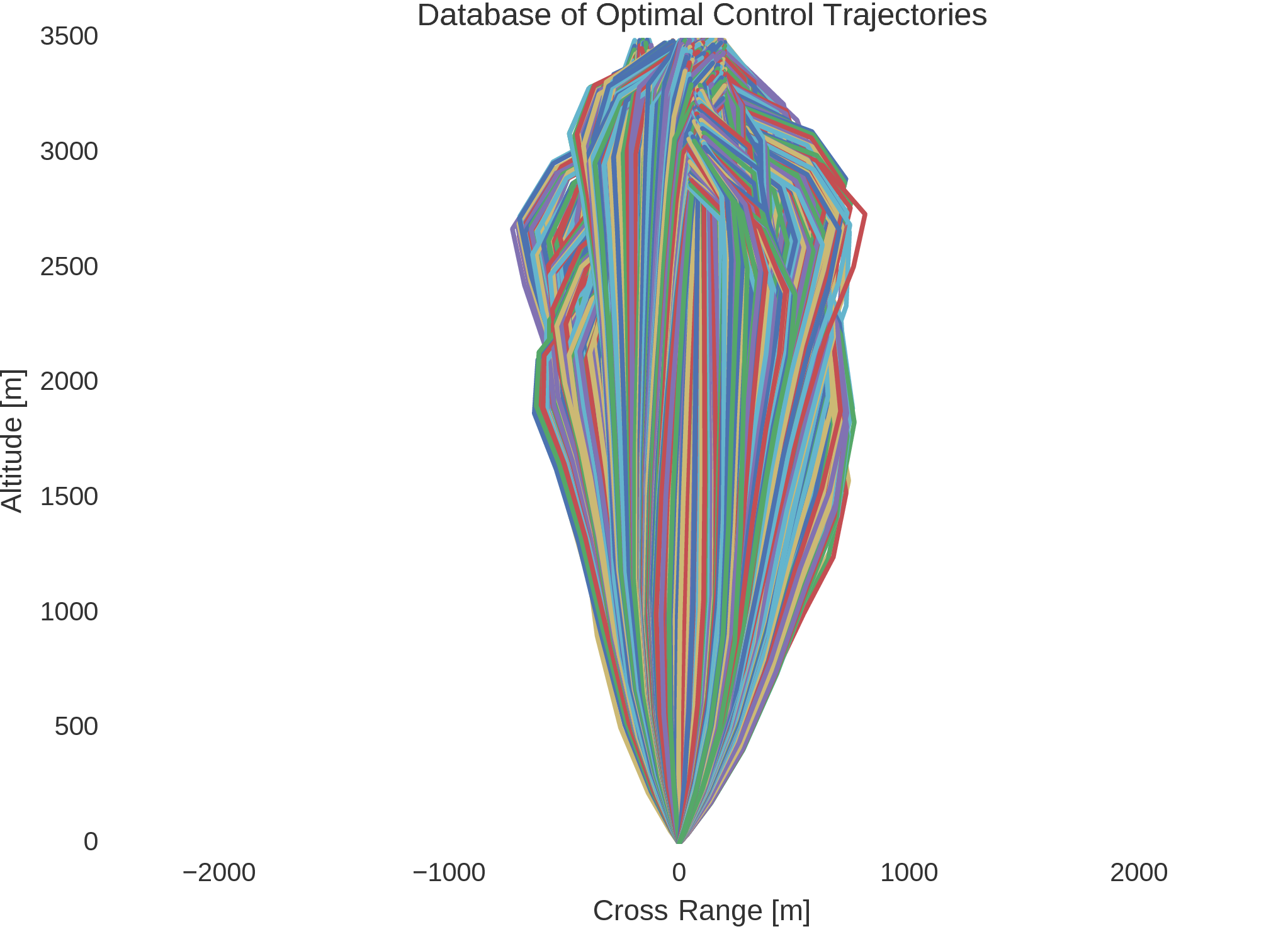
It is noted that this system’s control actions are similar to that of the simple point mass lander, and that the system’s dynamics prove to be sufficiently difficult in the analytical derivations required for indirect trajectory optimisation methods. As such, using the advantage of the topological continuation of the system’s dynamics, the Hermite-Simpson-Separated method is used to generate a large database of optimal control trajectories, with eight thousand generated optimal control trajectories, each with ten transcription segments enforced by the Hermite-Simpson quadrature and interpolation constraints. The state-control pairs along each of the generated trajectories are compiled into a single unified dataset, which forms 176000 samples, well over enough to sufficiently train artificial neural networks of especially deep architectures.

Neural Networks

Artificial neural networks are a modelling regime motivated by the structure and behaviour of the central nervous system in animals. Neural networks are popularly used for nonlinear modelling, forecasting, regression, and classification, and they quite often surpass the performance of advanced modelling and forecasting methods of other regimes.

Biomimetics

The structure of neural networks resemble a horde of connected artificial neurons that serve to emulate local memory which, from each neuron, is disseminated to other neurons. While the exact mechanism by which biological neural networks are trained is relatively unknown, in artificial neural networks there typically exists a training rule whereby weights of connections are iteratively manipulated through experience or by evidence in data. While the mechanism by which these manipulations are done more closely resembles that of numerical optimisation, the process conceptually represents that of which is seen in nature, for example a child learning to categorise the sentiment of their parents’ facial expressions. One of the most exciting merits of using artificial neural networks is their ability to generalise outside the domain in which they were trained. That is, a sufficiently trained neural network should be able to successfully infer correct results from unseen cases.

Training and Architecture

Artificial neural networks have shown a great deal of success in such tasks as classification, regression, and clustering. In this work focus is placed on supervised learning through regression.. In the process of supervised learning, a training pattern, consisting of corresponding input and output data, is attempted to be modelled by a function mapping inputs to outputs. Such a mapping function is represented, in this case, by a neural network, a nonlinear combination of parameters. The successful mapping of input data to output data is typical possible given enough data and computing resources, but especially powerful approximations models are fostered when the architecture of the implemented neural network includes at least one hidden layer.

Artificial neural networks are noted to be among the most effective methods for nonlinear regression. The learning process of neural networks, by which they iteratively learn the correct policy for mapping inputs to outputs, is characterised by the objective of minimising an error function with respect to a set of free parameters. One of such error functions is the commonly used mean squared error.

In recognising the merit of using deep artificial neural networks for nonlinear regression, in this software framework it has been made convenient to construct neural networks with one or more hidden layers, which find themselves amidst the burgeoning field of deep learning. One can easily instantiate a deep artificial neural network, again in a convenient object orientated approach, with three hidden layers, each layer having a user specified number of nodes.

'''
This net has 3 hidden layers.
Layer 1 has 10 nodes,
Layer 2 has 25 nodes,
Layer 3 has 5  nodes.
'''

layers = [10, 25, 5]
...
Neural_Net = MLP(path)
Neural_Net.build(data, iin, iout, layers)
...

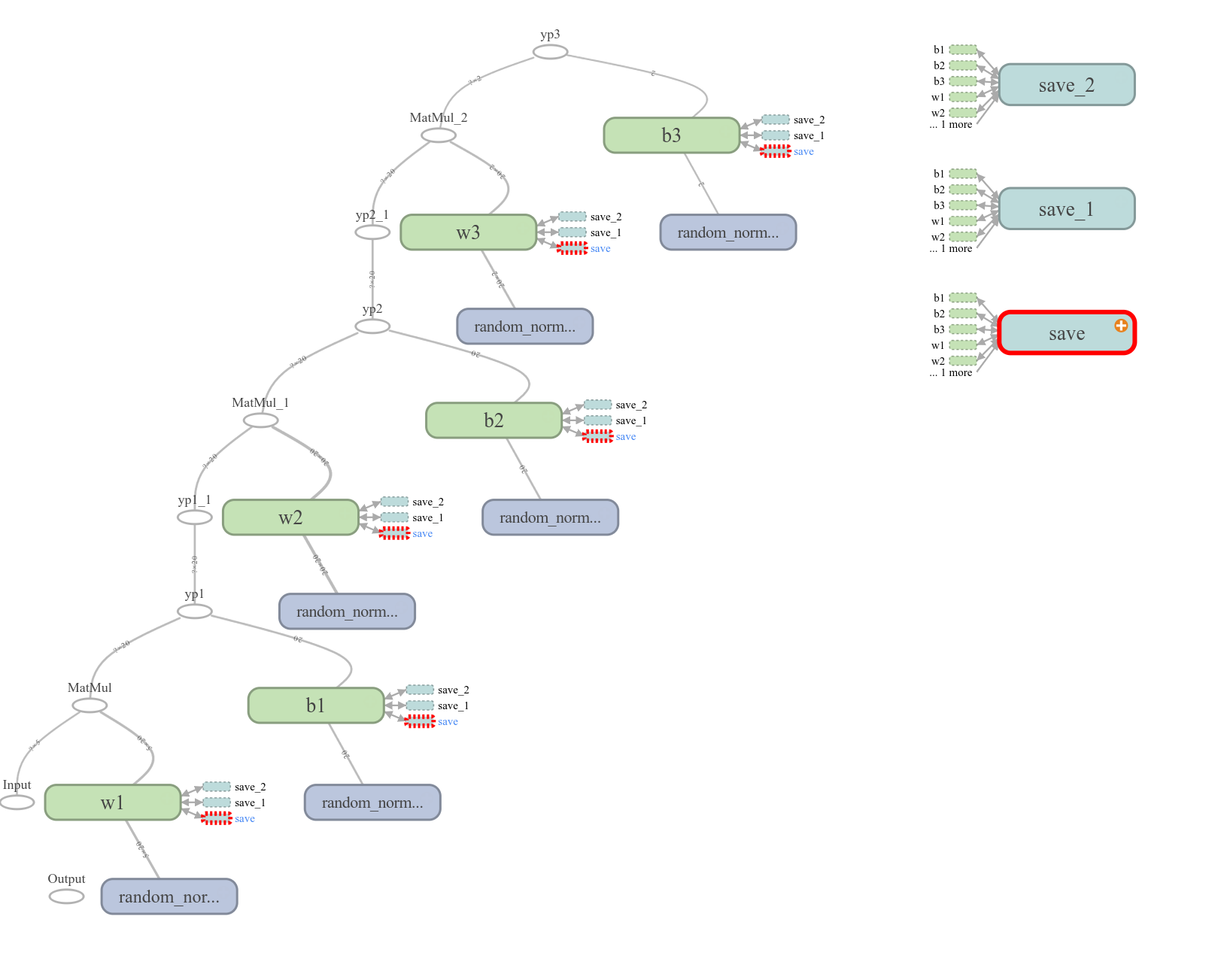
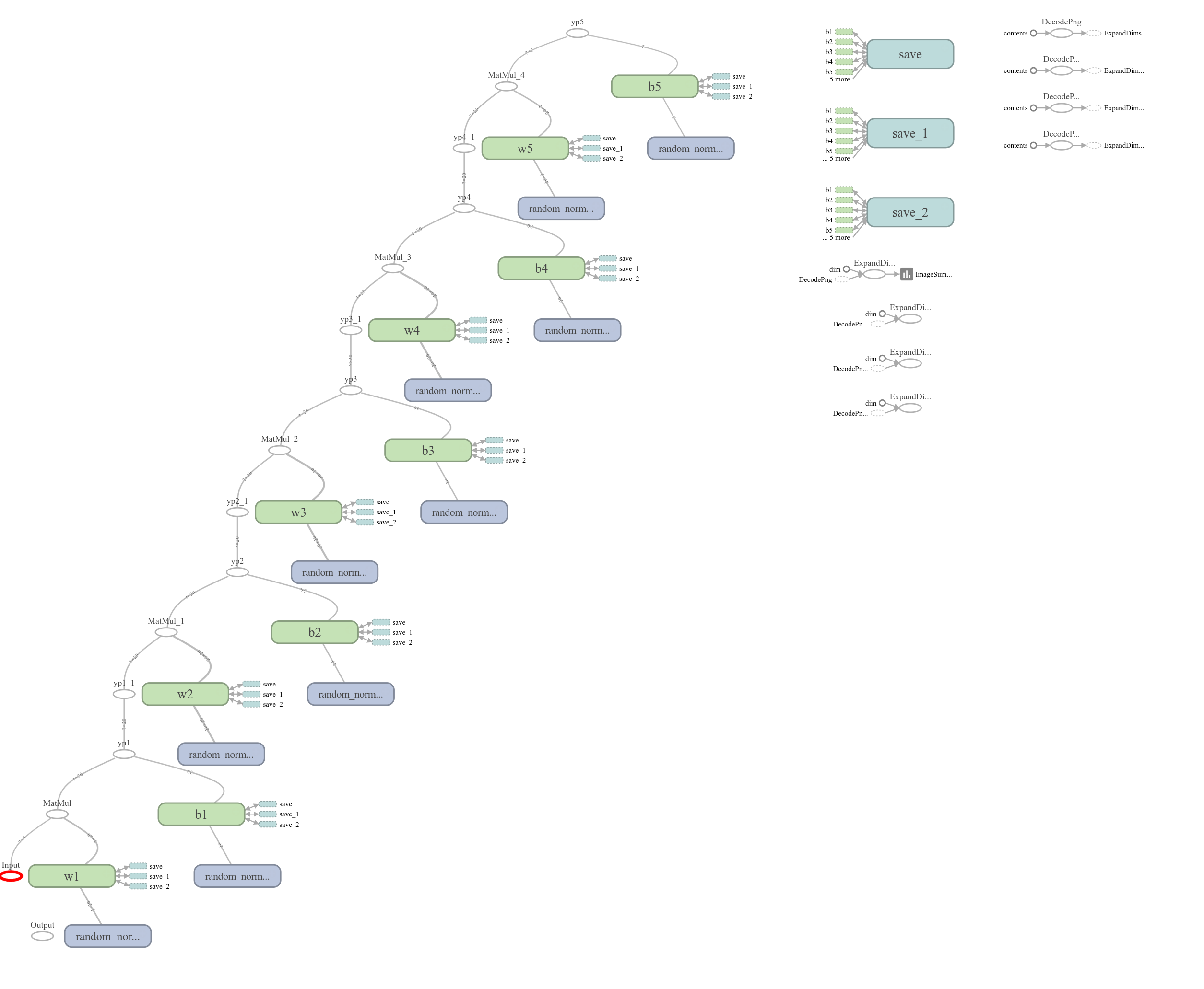
For example, one can see the visual architecture of a neural network with two hidden layers, each with twenty nodes ($20\times2$); and one with four hidden layers, each also with twenty nodes ($20\times4$).

Although it has long been pointed out that artificial neural networks with hidden layers form powerful models of nonlinear functional relationships, an algorithm to train such a network was, for quite some time, non-existent. The most significant challenge that prevented the finding of an appropriate training algorithm was that there was no way to judge the error produced within hidden layers; however, after many years the back propagation algorithm was spawned.

However, in this work, rather than the widely used back propagation algorithm, the Adam method of stochastic optimisation is used. The Adam method is a first-order gradient-based optimisation algorithm of stochastic objective functions, based on adaptive estimates of lower-order moments. This method is noted to be easy to use, computationally efficient, have little memory requirements, is invariant to diagonal rescaling of gradients, and is suited well for problems that entail large datasets and/or parameter spaces. Additionally, the need to worry about the behaviour of the learning rate of the model is circumvented, as the learning rate is theoretically guaranteed to decay in accordance to

where $\alpha$ is the nominal user specified learning rate and $t$ is the training iteration.

This algorithm is often regarded as state of the art in comparison to the back propagation algorithm, and hence its use is justified. Although the decay of the learning rate is taken care of, the nominal learning rate must be selected carefully. In the case of this optimal control trajectory database, the training progress of minimising the mean squared error to the model approximations is shown for multilayer perceptrons of architectures having

• two twenty node hidden layers ($20\times20$)
• four twenty node hidden layers ($20\times20\times20\times20$)
• four fifty node hidden layers ($50\times50\times50\times50$)

at a nominal learning rate of $\alpha=1\times10^{-2}$ and $\alpha=1\times10^{-4}$.

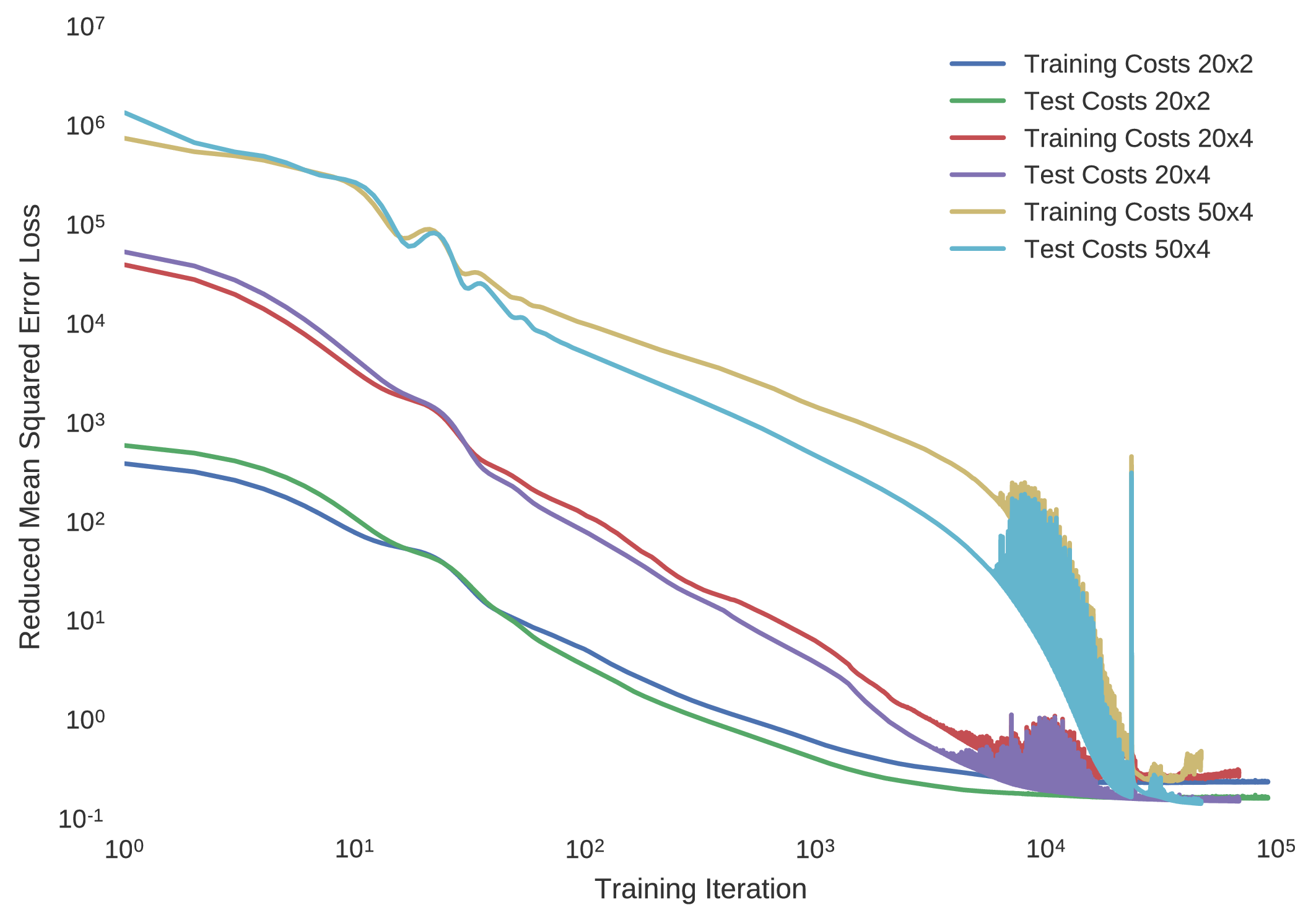
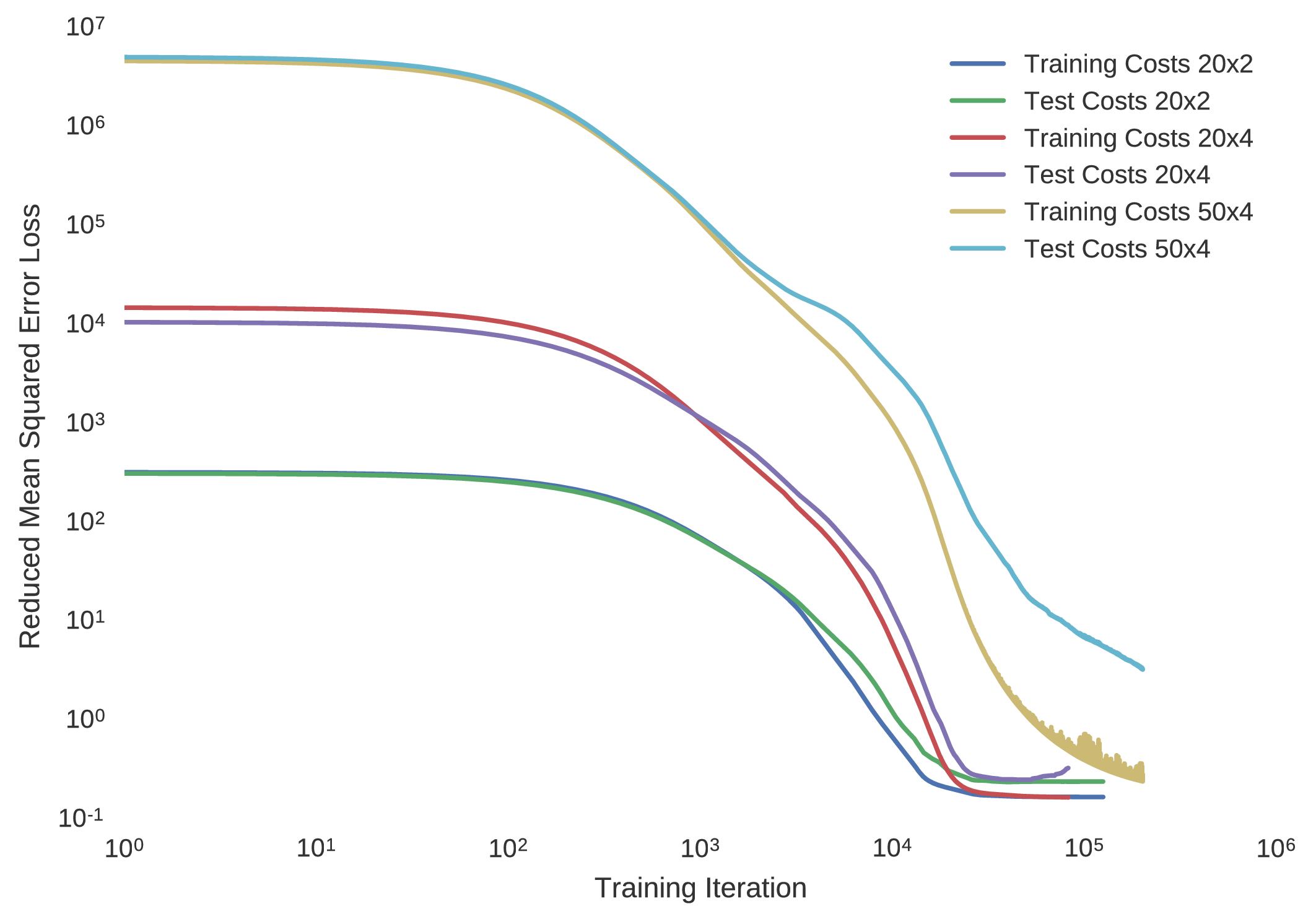
Indeed, it is seen that if the learning rate is set too greedily, the training convergence of the cost minimisation becomes rather noisy, hence improvement is seen with a more conservative learning rate. Despite this distinction, although a lower learning rate further encourages convergence to the true optimal network parameters, it does however result in a longer training duration, making it infeasible for many domestic computing apparatuses.

It has been shown with multi-layer perceptrons having a single hidden layer that including an excessive number of neurons typically results in over training. In the case of over-training, the implemented neural network is unable to generalise sufficiently. Although historically it was commonplace to iteratively manipulate a neural network’s number of nodes until a sufficient level of generalisation is achieved, it is now deemed more practical to implement early stopping, in which one halts the training of the subject neural network before it begins over-training. Thus at the expense of a more scientifically based method of determining a neural network’s structure, a large amount of time is saved by disregarding the neural network’s structure above a certain tolerance of sufficiency, determined through trial and error.

In this framework, users can interrupt and resume the training of a neural network at any moment without jeopardising the storage of the model’s parameters, as such parameters are saved at every training iteration for finalisation or later use. In order to investigate neural networks of various architectures, several multilayer perceptions can be conveniently analysed for the application of optimal control in parallel. Within this software framework, one can train multiple neural network architectures asynchronously.

from ML import MLP

def train(width, nlayers):
    ...

    # Instantiate the neural network
    net   = MLP(path)
    # Build the neural network
    net.build(data, iin, iout, layers)
    # Specify the learning rate
    lr    = 1e-4
    # Number of training iterations
    tit   = 200000
    # How often to display cost
    dispr = 300
    # Train the network
    net.train(lr, tit, dispr)
    ...

if __name__ == "__main__":
    nlayers = [1, 2, 3]
    width   = [10, 20]

    # Train asynchronously in parallel
    for args in itertools.product(width, nlayers):
        p = multiprocessing.Process(target=train, args=args)
        p.start()

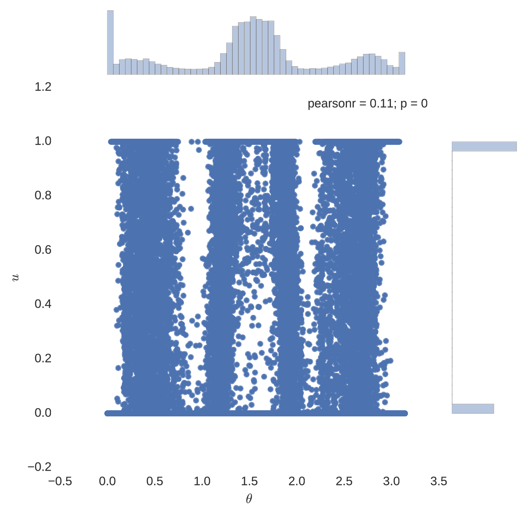
The success of using artificial neural networks to learn the optimal control polices of dynamical systems is indeed seen, with all implemented neural network models plateauing to a mean squared error loss of approximately $e\approx0.16$ for the Mars lander dynamical system. In particularly deep neural architectures, such as those implemented here, rectified linear units used as nodal activation functions are seen to indeed avoid the problem of vanishing gradients that come with additional layers, imparted by the saturating tendencies of sigmoidal units. Indeed, it is seen that the expected bang-bang policy of optimal control theory is mimicked in accordance to the figures below, where it is noted that the network having a greater number of hidden layers seems to more coherently replicate the expected policy.

Neuro-Control

Assuming that the user’s implemented artificial neural network model has been properly trained, it is easy for users to implement their neural network model to directly control their unique dynamical model between a chosen initial and final state. Different neural network architectures are easily examined in their success to meet specified boundary conditions with this framework’s object orientated approach. In this section, artificial neural networks of architectures $20\times2$ and $20\times4$, are examined in their ability to not only control the user defined dynamical system within the training domain, but also generalise their learnt optimal control policy outside of the region in which they have been trained. The process of implementing trained artificial neural networks to control the user’s own dynamical model as follows.

# Select randomly a few training trajectories
itraj = np.random.choice(range(ntraj),10)
test_si = data[itraj,0,0:5]
# Instantiate the dynamical system
model = Point_Lander_Drag()
# The name of the trained neural network
net = 'HSS_10_Model'
# Shorthand dimension of the network
dim = (20, 4)
# Assign the neuro-controller to the system
model.controller = Neural(model, net, dim).Control
# Time of simulation
tf = 100
# The resolution of numerical integration
nnodes = 500
# Control the system from several initial states
for si in test_si:
    s, c = model.Propagate.Neural(si, tf, nnodes, False)
    t = np.linspace(0,tf, nnodes).reshape(nnodes,1)
    fs = np.hstack((s,c,t))
    fsl.append(fs)

In verifying the success of each neural network to optimally control the trajectory of a dynamical system, random initial states are typically selected within the 5% dilated box-bounded region in which the training initial states were generated from. From the randomly selected initial states the dynamics of the system are then propagated with the control mapping enforced by the implemented neural network. Ten neuro-controlled trajectories are shown for the $20\times2$ and $20\times4$ neural networks in regard to position and thrust throttle profile.

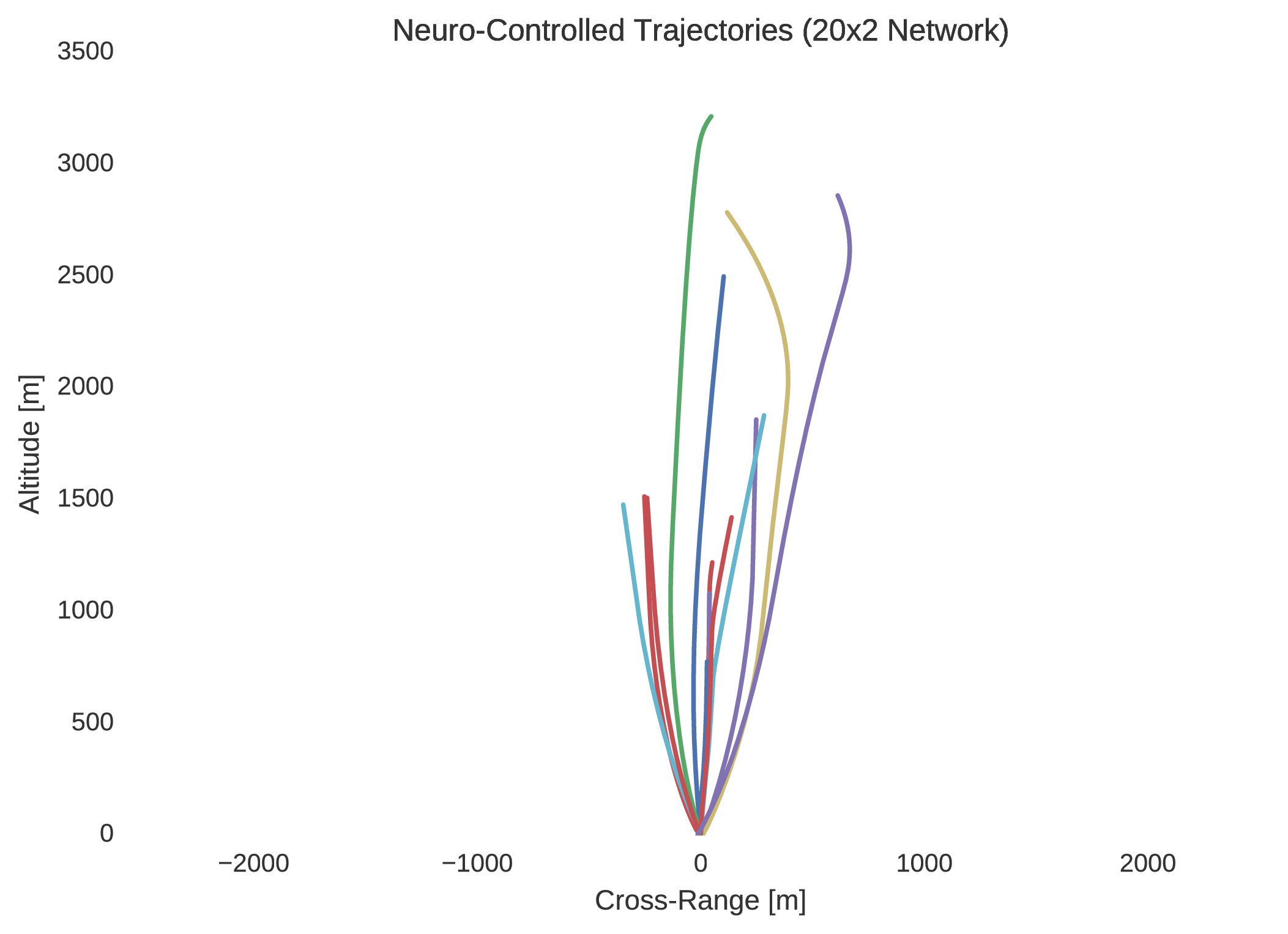
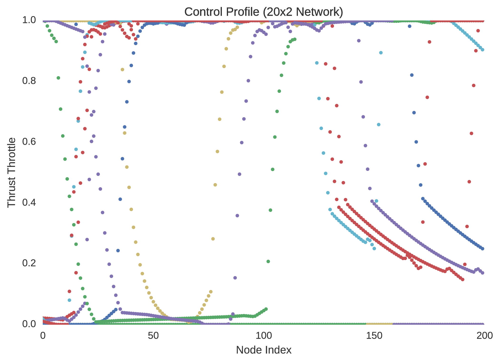
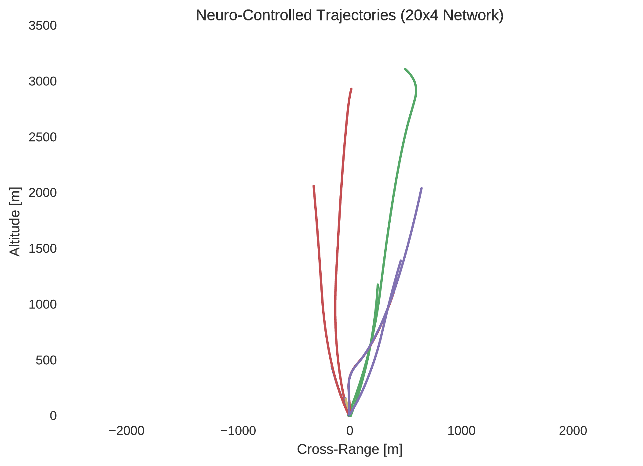
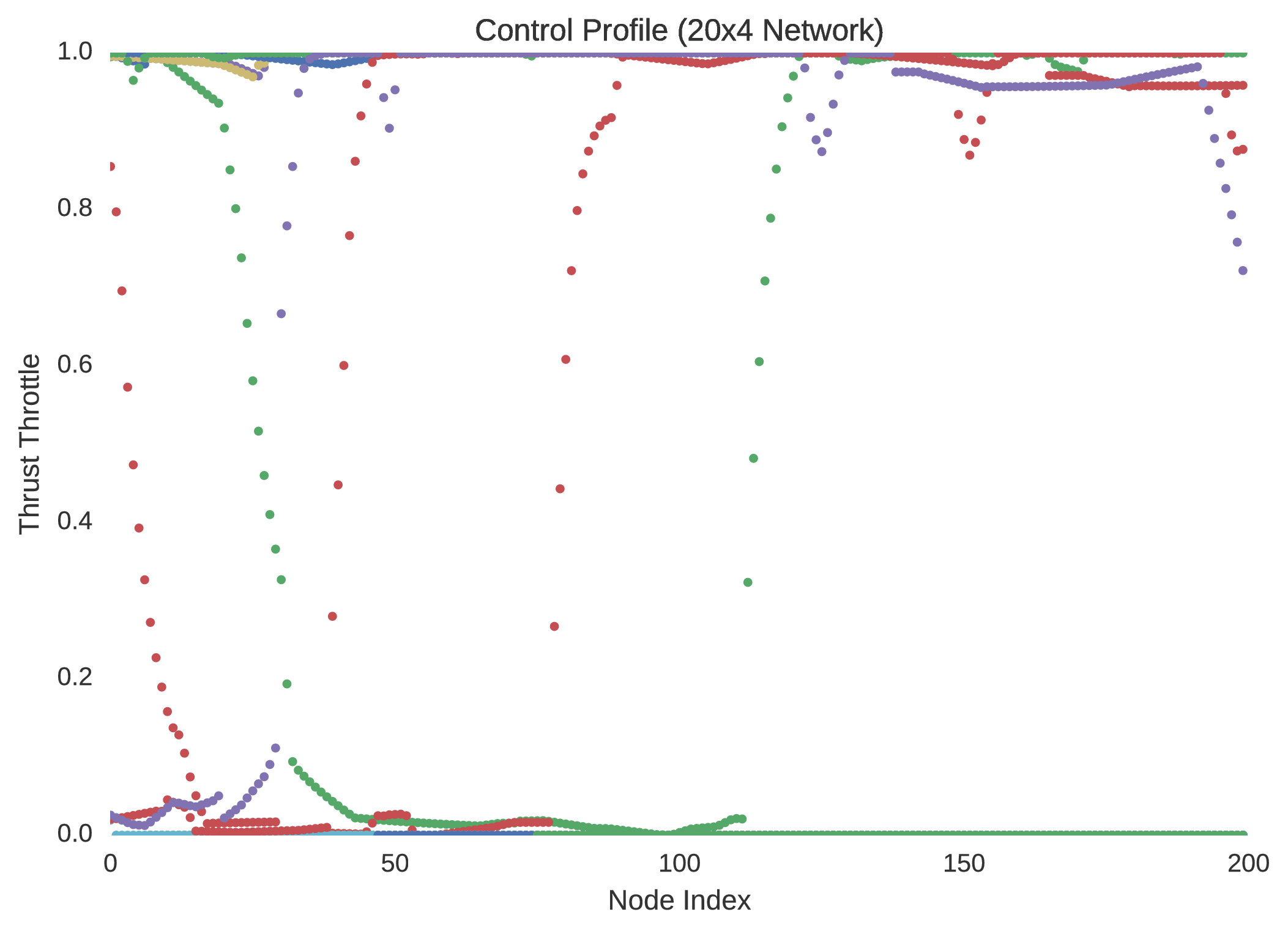
Indeed, it is quite easily seen that the $20\times4$ network is superior to the $20\times2$ network in performance. Not only is this evidenced by the network’s regression of the training database, but more importantly by its performance with respect to its dynamic implementation as a real-time controller. The difference between the control profile generated from the $20\times2$ network and the $20\times4$ network is revealing; the $20\times4$ network is more accurately able to replicate the bang-bang optimal control profile that was to be expected in accordance to optimal control theory. This is unsurprising as it is widely indicated in the field of machine learning that the addition of extra hidden layers to an artificial neural network increases significantly its ability to generalise its behaviour to unseen scenarios outside the domain in which it was trained.

Indeed, by simulating the controlled trajectories imparted by the $20\times2$ and $20\times4$ networks, the advantage of additional layers is exemplified. Although the optimal control data generated through nonlinear programming is accurate, it is not entirely precise, as there exists so called chattering effects due to the discretisation of the system’s state-time dynamics. Despite this, while it is not guaranteed that such a neural network’s control will prove to be capable of mass-optimal control, it is shown that they would indeed be able to control such a system with sufficient feasibility. That is, although the neuro-controlled dynamical system may not perfectly exploit its environmental dynamics to maximise its savings with respect to fuel expenditure, as would be expected from global trajectory optimisation, it should indeed be able to safely land. Thus, in this respect, such neuro-controllers as those explained in this text, present the significant capability to autonomously control such dynamical systems in real-time.

Going Forward

It is shown that neural networks trained on optimal state-control pairs enables the real-time implementation of optimal control. It is shown that these intelligent controllers may pose a substitution for the popular usage of controllers that used linear dynamics about a nominal trajectory. Using neural networks as controllers enables appropriate control outside of a nominal trajectory, thus making them more robust to anomalies than the currently implemented controllers.

It has been shown in this work that supervised learning poses merit for use in real-time optimal control. Comparing this method to reinforcement learning, it is noted that a significant advantage is that the user does not have to manually assign reward to an environment, which for the application of crucial aerospace control, seems rather arbitrary. Supervised learning requires data, which in new scenarios may not be readily available. However, considering the plethora of data in this now data-driven world, supervised learning proposes a great deal of merit. Considering these points, a strategy of exploiting each regimes merits is sought.

A potential direction of future work is to combine the merits of both reinforcement and supervised learning in what is known as guided policy search. This method essentially employs reinforcement learning in regular practice; However, instead of manually assigning rewards to an environment, optimal examples are given through trajectory optimisation, hence the benefits of both reinforcement learning and supervised learning are combined, with their drawback being eliminated.

General Artificial Intelligence

It would also be interesting to develop a general methodology for the intelligent control of such systems as the one analysed here, not only to optimally control themselves with respect to a specific objective while satisfying constraints, but also to develop a more general sense of intelligence. Investigating the ability of such systems to extract knowledge from explorative interactions with their environment and investigate how these discoveries manifest their advantages within new objective regimes and different systems may harbour significant findings. By investigating a system’s ability to discover knowledge from interacting with its environment, and exploring how it behaves under certain objectives, a generalised framework could be developed to draw interconnections between these regimes, resulting in a closer representation of generalised intelligence. Given this field’s rapidly developing and highly interdisciplinary nature, cutting-edge findings from all areas of intelligent systems will be embraced to strengthen these research efforts.