STOCHASTIC SHAPE OPTIMISATION OF UAV WING UNDER UNCERTAINTY

Christopher Iliffe Sprague


ABSTRACT

This paper examines the design of a wing for a new long-endurance aircraft that will be used as a telecommunications platform. In particular, the problem of optimizing the shape of the wing’s spar, acting as the aircraft’s main structural support, in order to minimize its mass, is analyzed and solved. In doing so, a robust object-orientated programming approach is taken to transcribe the problem and flexibly find optimal solutions from user defined design guesses. Using a complex step finite difference method and stochastic collocation, the geometry of the wing’s spar is optimized with respect to its mass, under uncertain loading conditions. It is shown that a design mass of %70 percent lower than the nominal is feasible.

Index TermsWing Structure, Shape Optimization

Contents

1 Problem Model
 1.1 Specifications
 1.2 Problem Formulation
 1.3 Geometrical Parametrization
  1.3.1 Design Vector
  1.3.2 Spanwise Location
  1.3.3 Volume and Mass
 1.4 Material Stress Constraints
  1.4.1 Load Distribution
  1.4.2 Second Moment of Area
  1.4.3 Displacement and Stress
 1.5 Manufacturing Constraints
  1.5.1 Radii Bounds
  1.5.2 Thickness
2 Optimization
 2.1 Sequential Quadratic Programming
 2.2 Objective and Constraint Gradients
  2.2.1 Forward Difference
  2.2.2 Central Difference
  2.2.3 Complex Step
3 Results
 3.1 Source Code

List of Tables

Problem Specifications

List of Figures

Spanwise Linear and Perturbed Force Distributions
Nominal Stress Statistics with 20 Nodes
Complex Step Convergence with 25 Nodes and 3 Collocation Points
Complex Step Convergence with 25 Nodes and 5 Collocation Points
Complex step convergence
Optimized Design with 25 Nodes and 3 Collocation Points
Optimized Design with 25 Nodes and 5 Collocation Points
Optimized Geometry
Optimized Stress Statistics with 25 Nodes and 3 Collocation Points.
Optimized Stress Statistics with 25 Nodes and 5 Collocation Points.
Optimized Stress Statistics

Listings

1 Problem Model
 1.1 Specifications
 1.2 Problem Formulation
 1.3 Geometrical Parametrization
  1.3.1 Design Vector
  1.3.2 Spanwise Location
  1.3.3 Volume and Mass
 1.4 Material Stress Constraints
  1.4.1 Load Distribution
  1.4.2 Second Moment of Area
  1.4.3 Displacement and Stress
 1.5 Manufacturing Constraints
  1.5.1 Radii Bounds
  1.5.2 Thickness
2 Optimization
 2.1 Sequential Quadratic Programming
 2.2 Objective and Constraint Gradients
  2.2.1 Forward Difference
  2.2.2 Central Difference
  2.2.3 Complex Step
3 Results
 3.1 Source Code

1.

1 Problem Model

1.1.

1.1 Specifications

Preceding the construction of the optimization problem, it is necessary to define the constant metrics that characterize the nature of the problem. For the case of an annular spar, the problem parametrization requires several design metrics to be taken into account, namely: wing semi-span L, material density ρ, Young’s modulus E, ultimate tensile/compressive strength σmax, aircraft operational mass M, minimum spar thickness Tmin, minimum inner wall radius rmin, and maximum outer wall radius Rmax.

Additionally, the operational conditions that the aircraft will be subjected to need to be taken into account, namely: gravitational acceleration g, and maximum operational G-force G. In this particular investigation, attention will be directed towards the case of a carbon fiber spar, whose specifications are enumerated in Table 1. One can instantiate a UAV of this nature through an object-oriented approach, as shown in Listing 1. The full source code of the UAV class is shown in Listing 5.


Listing 1: UAV Instantiation
% Instantiate the wing 
Raptor = UAV(... % With properties: 
  7.5,       ... % Wing semi-span [m]. 
  1600,      ... % Spar density [kg/m^3]. 
  7e10,      ... % Modulus of elasticity [Pa]. 
  600e6,     ... % Maximum spar strength [Pa]. 
  500,       ... % Mass of aircraft [Kg]. 
  9.807,     ... % Earth's gravity [m/s^2]. 
  2.5e-3,    ... % Minimum spar thickness [m]. 
  1e-2,      ... % Minimum inner spar radius [m]. 
  5e-2,      ... % Maximum outer spar radius [m]. 
  2.5,       ... % Maximum operational G-force. 
  5,         ... % Number of collocation points. 
  4          ... % Number of perturbations pts. 
  );


Table 1: Problem Specifications


Parameter SymbolValue


Semi-Span L 7.5 m


Density ρ 1600 kg∕m3


Young’s Modulus E 70 GPa


Ultimate Strength σmax 600 MPa


Aircraft Mass M 500 kg


Minimum Thickness Tmin 2.5 mm


Minimum Inner Radius rmin 1 cm


Maximum Outer RadiusRmax 5 cm


Gravity g 9.81 m∕s2


G-Force G 2.5


1.2.

1.2 Problem Formulation

The objective of this optimization problem is to minimize the total mass of the spar through structural alteration, while not allowing its structural stress σ at any spanwise location to exceed its material’s ultimate strength σmax during its maximal operational loading conditions. In this particular optimization process, the uncertainty of the wing’s load distributions is taken into account. That is, the stress constraint of the spar becomes the wing’s average stress plus six standard deviations. This statistical constraint characterization is discussed further in Section 1.4.1. Additionally, there are also manufacturing constraints that dictate the spar’s inner radius r and outer radius R to satisfy r rmin and R Rmax, while satisfying a thickness constraints R - r Tmin. In a more formal manner, this problem’s formulation is shown as:

m inimize  m(R ) | R ↦→ {r(x),R(x)} | x ∈ [0,L]
   R
subj∀ecxtto  rmin ≤ r(x) ≤ rmin + Tmin
          R    - T   ≤ R (x) ≤ R
           max    min           max
          r(x)- R (x) ≤∘- Tmin-----
          E(σ(x,ξ))+ 6  V ar(σ (x,ξ))- σmax ≤ 0
Essentially, the annular spar’s inner and outer spanwise radii {r(x),R(x)} must be manipulated until the spar’s total mass m(R) has reached a minimum value for all possible satisfactory forms of r(x) and R(x).

1.3.

1.3 Geometrical Parametrization

Because finite element methods will be used to solve this optimization problem, it is required to discretize the spar’s geometry into a series of spanwise finite elements. Herein, the wing’s spar will be represented by a series of nodes, indexed by i, where i = 1 and i = n signify the locations of the wing’s root and tip respectively. As such, it can be deduced that there are n nodes and n- 1 finite elements along the span of the spar. Hence, the set of node indexes N and finite element indexes E are defined as follows

  N = [i,i+ 1,...,n]

E = [j,j + 1,...,n- 1]

1.3.1.

1.3.1 Design Vector

It is appropriate to begin the optimization process with the formulation of the design vector R, composed of inner radii r and outer radii R. Abiding to the form of a column vector, it is necessary to apply a change of variables and define the design vector as follows,

  R = [ξk,ξk+1,...,ξ2n]T

{ξ2k-1,ξ2k} ← {ri,Ri}∀i ∈ I
It can be seen that the inner and outer radii are sequenced to occur for every other index in the design vector R.

1.3.2.

1.3.2 Spanwise Location

Having deduced the number of nodes n from the user supplied design vector, the spanwise location along the spar can be discretized in a similar manner as,

x = [xi,xi+1,...,xn] | x1 = 0,xn = L
, where it is noted that the first and final index values of xi satisfy the length of the wing’s semi-span.

1.3.3.

1.3.3 Volume and Mass

At each node i along the wing’s span, the spar’s cross section is represented as a circular annulus of inner and outer radii, ri and Ri, respectively, whose area is defined by Ai = π(Ri2 - ri2). Assuming this cross sectional area characterization is consistent across all nodes, the inner and outer surfaces of each finite element j are linearly interpolated between their corresponding nodes i = j and i = j + 1. Hence the nodes’ cross sectional areas are integrated along the interpolations, yielding the volume of each finite element as follows

Vj = π-(r2j- R2j+rjrj+1- RjRj+1+r2j+1- R2j+1)(xj- xj+1)
     3
As such, the total volume of the spar can be computed by a summation across all finite elements V = j=1n-1V j. Subsequently the spar’s total mass is obtained as m = ρV , and hence the optimization problem’s objective function m(R).

1.4.

1.4 Material Stress Constraints

As formulated in Section 1.2, the structural stress at any spanwise location along the spar must not exceed its material’s ultimate strength, σi - σmax 0 i I. Modeling the wing’s spar as a cantilever beam, Euler-Bernoulli beam theory can be exploited to compute the spar’s nodal stress.

1.4.1.

1.4.1 Load Distribution

In this study, a linear load distribution is no longer assumed. Rather, the force distribution experienced by the aircraft’s spar is formulated as the nominal linear force distribution plus a probabilistic perturbation given by

         4      (          )
δ(x,ξ) = ∑  ξ cos (2n---1)πx-
       n=1  n        2L
with ξn ~N(       )
 0, fno1m0(n0). Hence the force along the wingspan can be formulated as
F (x,ξ) = GM--g(1 - xi)+ δ(x,ξ)
           L       L
. With the specifications given in Table 1 and Listing 1, the nature of the spar’s perturbed force distribution can be seen in Figure 1.


Fig. 1: Spanwise Linear and Perturbed Force Distributions

PIC


1.4.2.
1.4.2 Second Moment of Area

In order to calculate the displacement of the spar at any location along its span, the second moment of inertia at each node must first be calculated. For a circular annulus describing the cross section of any node along the spar’s span, the second moment of area is formulated as such

    π ( 4   4)
Ii = 4 Ri - ri

1.4.3.

1.4.3 Displacement and Stress

Assuming a transversely applied load distribution and cross sectional symmetry, a cubic Hermite finite-element basis is used to solve the Euler-Bernoulli beam equations. The vertical and angular displacement of the spar at each node along the beam are calculated, using the aforementioned formulations of the load distribution and second moment of area. The beam’s vertical displacement is formulated as follows δ = [δii+1,n]T. Using the spar’s displacements, its nodal tensile stresses are computed and formulated as such σ = [σii+1,n]T. Hence the constraint function must satisfy the following

        ∘ -------
E(σi)+ 6  Var(σi)- σmax ≤ 0∀i ∈ I
Using stochastic collocation and Gauss-Hermite quadrature, with the 4 uncorrelated Gaussian random variables indicated in Section 1.4.1, the mean stress is computed as
           (          )          (      )
             ∏4   1     ∑m    m∑   ∏4
E (σ(x,ξ)) =     √2-πσn-    ⋅⋅⋅       win
             n=1         i1    i2  n=1
Within the loop of computing the expected stress value, the standard deviation is computed as well, with the following formulation
∘ -----------  ∘ ----------------------
  Var(σ(x,ξ)) =  E(σ(x,ξ)2) - E (σ(x,ξ))2
. The nominal statistics for the average expected stress distribution can be seen in Figure 2

PIC

Fig. 2: Nominal Stress Statistics with 20 Nodes


The unadjusted abscissas and weights corresponding to the m collocation points are computed through the Gauss-Hermite subroutine given in Listing 2.

Listing 2: Gauss-Hermite Abscissas and Weights
function [xi, w] = GaussHermite(obj,n) 
    % Computes abscissas x and weights w 
    % for Gauss-Hermite quadrature of order n 
    i   = 1:n-1; 
    a   = sqrt(i/2); 
    % Use a diagonal matrix for real roots 
    CM  = diag(a,1) + diag(a,-1); 
    % V = column eigenvectors 
    % D = diagonal matrix of eigenvalues 
    [V D]   = eig(CM); 
    % Get abscissas 
    [xi i] = sort(diag(D)); 
    V       = V(:,i)'; 
    % Weights 
    w       = sqrt(pi)  V(:,1).^2; 
end

For further background on the derrivation of this method, the reader is advised to consult [?]. 1.5.

1.5 Manufacturing Constraints

As required by the optimization problem’s specifications, the inner and outer radii of each annular cross section cannot be less than Tmin apart, the inner radius cannot be smaller than rmin, and the outer radius cannot be larger than Rmax.

1.5.1.

1.5.1 Radii Bounds

In formulating the range to which the inner radii ri and outer radii Ri are bounded, it is necessary to formally define lower and upper bound vectors L and U, respectively, that satisfy L R U, corresponding to the form of the transformed design vector R described in Section 1.3.1. The lower and upper bounds for the radii, corresponding to the constraints described in Section 1.2, are formulated as such

 L = [λk,...,λ2n]T | {λ2k-1,λ2k} ← {rmin,rmin +Tmin}
U = [υ ,...,υ  ]T | {υ  ,υ  } ← {R    - T   ,R   }
      k     2n      2k- 1 2k      max    min  max

1.5.2.

1.5.2 Thickness

In order to enforce the constraint that the annular spar’s wall thickness may not be smaller than Tmin and that the outer radii must always be greater than the inner radii Ri > ri i I, linear inequality constraints must be instantiated. In doing so, it is required to formulate a n × 2n matrix A and n × 1 column vector b that satisfy AR b. The matrices are defined as follows

    ⌊               ⌋
      αi,k  ⋅⋅⋅  αi,2n
A = |⌈  ...   ...   ...  |⌉ | {αi,2i-1,αi,2i} ← {1,- 1}
      α    ⋅⋅⋅ α
       n,k        n,2n  T
         b = [βi,...,βn]  | βi ← - Tmin
where R is defined as the 2n × 1 column vector described in Section 1.3.1. For further information on formatting constraints and objectives to accommodate Matlab’s built in functions, the reader is advised to consult [?].

2.

2 Optimization

2.1.

2.1 Sequential Quadratic Programming

Sequential quadratic programming (SQP) has proven itself as one of the most successful methods for solving nonlinearly constrained optimization problems. Essentially, SQP aims to model the nonlinear programming problem (NLP) at a given approximate solution Rh by a quadratic programming subproblem, then use the subproblem to construct a better approximation Rh+1. This process is iterated until convergence to a solution R* is achieved. SQP is not a feasible point method; neither the point nor any of the subsequent iterates are required to be feasible. However, the SQP method does satisfy the bounds L and U at every iteration, and is ideal for small to medium scale problem such as in the case of this paper’s optimization problem, where optimality returns are generally diminished for n > 40. This method of nonlinear constrained optimization is handled natively by Matlab’s fmincon function [?], and described in more detail in [?].

2.2.

2.2 Objective and Constraint Gradients

In order to achieve an optimal design vector R* that satisfies m(R*) m(R)R↦→{ri,Ri}∀i I, both the necessary and sufficient conditions for optimality need to be realized. It is necessary for an optima at a stationary point R to have a first derivative of zero R = 0. It is sufficient to call the stationary point a local minimum R* if 2R* > 0. For further information on conditions of optimality, the reader should consult [?].

2.2.1.

2.2.1 Forward Difference

Among the simplest methods of finite difference derivative approximations is the forward step method

          f(R + hiei)- f(R )
∇ ξif(R ) =-------hi--------+ O(hi)
, where ei represents a vector of zeros with the ith index equal to 1, O(hi) represents the truncation error, and hi represents the step size. Herein, hi represents the positive distance from |ξi| to the next larger floating-point number of the same precision as ξi. It should be noted that f may represent either the problem’s objective function m(R) or constraint function c(R).

2.2.2.

2.2.2 Central Difference

Similarly to the forward difference method, the approximate derivative of either the objective or constraint functions may be approximated with a perturbation to the design vector R. Under the central difference paradigm, the finite difference derivative approximation becomes

          f(R + hiei)- f(R - hiei)
∇ ξif(R ) =---------------------- +O (h2i)
                    2hi
It should be noticed that the central difference method is second-order accurate since the dominate term in its truncation error is O(hi2). Therefor the central difference method is more accurate than the forward difference method due to its smaller truncation error.

2.2.3.

2.2.3 Complex Step

Among the best of the finite difference methods is complex-step. It has shown to be very accurate, robust, and easy to implement, while maintaining a reasonable computational cost. The relationship between the real and imaginary parts of the function at hand is exploited to yield a derivative approximation of the following form

                     √---
          ℑ[f(R-+-hiei---1)]     2
∇ ξif(R) =        hi        + O(hi)

The complex step method converges quadratically with decreasing step size. This method is particularly advantageous because it is insensitive to small step sizes and eventually achieves the accuracy of its function evaluations. The reader can learn more about its derivation in [?]. Herein, focus will be directed towards the use of the complex step method to approximate the gradients of both the objective function m(R) and constraint function C(R). The complex step method can be formulated to approximate the functions’ Jacobian matrices as shown in Listing 3. As an example, to approximate the gradient of the objective function, one should execute obj.Complex_Jacobian(@obj.Stress_Constraints, R).


Listing 3: Complex Step Method
function jac = Complex_Jacobian(obj, funct, R) 
  fval = funct(R); 
  n    = numel(R); 
  m    = numel(fval); 
  jac  = zeros(m,n); 
  h    = eps(R)n; 
  for I=1:n 
    r        = R; 
    r(I,1)   = r(I,1) + h(I,1)i; 
    jac(:,I) = imag(funct(r))/h(I,1); 
  end 
  jac = jac.'; 
end

3.

3 Results

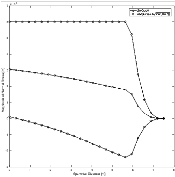
Having instantiated an aircraft with the specifications enumerated in Table 1, one can supply an initial guess to the optimizer. The initial guess of the 2n × 1 design vector R0 will characterize the nominal design of the spar’s radii, such that {ri,Ri}←{0.0415,0.05}∀i I, yielding an initial total spar mass of m0 = 29.32 kg. With the use of the complex step finite difference method and a varying amount of collocation points, the optimizer settled upon a final mass of m = 8.59221 kg, which is a %70.7026 decrease from the nominal mass, as shown through the convergence of the optimizer in Figure 4. The resulting spar geometries are seen in Figure 6. As one can see from Figure 8, the average stress and standard deviations are markedly different from the corresponding nominal plot in Figure 2. It is also seen throughout the figures that varying the number of collocation points did not affect the final optimal mass of the spar. It is seen that the new constraints enforced by the uncertainty model have made their effect known, as it is seen in Figure 8 that the six standard deviations above the mean stress have settled upon the constraint.
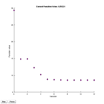

PIC Complex Step Convergence with 25 Nodes and 3 Collocation Points
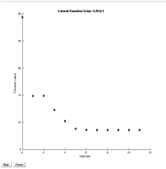
PIC Complex Step Convergence with 25 Nodes and 5 Collocation Points
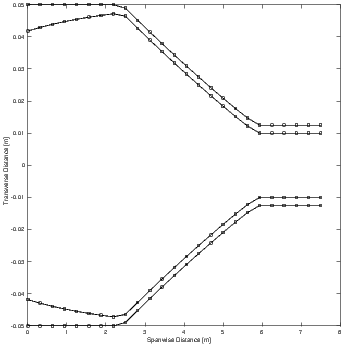
Fig. 4: Complex step convergence


PIC Optimized Design with 25 Nodes and 3 Collocation Points
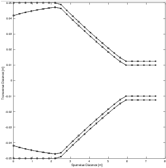
PIC Optimized Design with 25 Nodes and 5 Collocation Points
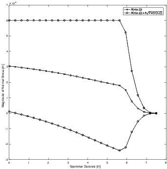
Fig. 6: Optimized Geometry


PIC Optimized Stress Statistics with 25 Nodes and 3 Collocation Points.
PIC Optimized Stress Statistics with 25 Nodes and 5 Collocation Points.

Fig. 8: Optimized Stress Statistics


3.1.

3.1 Source Code


Listing 4: UAV Optimization Example
 
clear all 
% Instantiate the wing 
Raptor = UAV(... % With properties: 
  7.5,       ... % Wing semi-span [m]. 
  1600,      ... % Spar density [kg/m^3]. 
  7e10,      ... % Modulus of elasticity [Pa]. 
  600e6,     ... % Maximum spar strength [Pa]. 
  500,       ... % Mass of aircraft [Kg]. 
  9.807,     ... % Earth's gravity [m/s^2]. 
  2.5e-3,    ... % Minimum spar thickness [m]. 
  1e-2,      ... % Minimum inner spar radius [m]. 
  5e-2,      ... % Maximum outer spar radius [m]. 
  2.5,       ... % Maximum operational G-force. 
  5,         ... % Number of collocation points. 
  4          ... % Number of perturbations pts. 
  ); 
 
% Take an initial guess of the spar's radii. 
R = zeros(80,1); 
for I=1:Raptor.N_Nodes(R) 
    R(2⋆I-1,1) = 0.0415; 
    R(2⋆I, 1)  = 0.05; 
end 
[x,fval,exitflag,output,lambda,grad,hessian] = Raptor.Optimize(R,'complex') 
Raptor.Plot_Stress_Stats(x)

Listing 5: UAV Class
 
classdef UAV 
    properties 
        Length;   % Wing semi-span [metres]. 
        Density;  % Density of spar [kg/m^3]. 
        E;        % Longitudinal modulus [Pascals]. 
        Strength; % Ultimate strength [Pa]. 
        Mass;     % Aircraft operational weight [Kg]. 
        Gravity;  % Gravity [m/s^2]. 
        Tmin;     % Minimum spar thickness [m] 
        Rimin;    % Minimum inner spar radius [m] 
        Romax;    % Maximum outer spar radius [m] 
        Gmax;     % Maximum operational G-force. 
        NCol;     % Number of collocation points. 
        NPert;    % Number of perturbation pts. 
    end 
 
    methods 
        function obj = UAV(L, dens, E, stren, m, ... 
                g, tmin, rimin, romax, Gmax,NCol,NPert) 
            % Constructs an instance of the UAV class. 
            obj.Length   = L; 
            obj.Density  = dens; 
            obj.E        = E; 
            obj.Strength = stren; 
            obj.Mass     = m; 
            obj.Gravity  = g; 
            obj.Tmin     = tmin; 
            obj.Rimin    = rimin; 
            obj.Romax    = romax; 
            obj.Gmax     = Gmax; 
            obj.NCol     = NCol; 
            obj.NPert    = NPert; 
        end 
 
        function NN = N_Nodes(obj, R) 
            % Returns the integer number of nodes 
            % according to the number of radii given. 
            NN = length(R)/2; 
        end 
 
        function NE = N_Elements(obj, R) 
            % Returns the integer number of finite 
            % elements. 
            NE = obj.N_Nodes(R) - 1; 
        end 
 
        function X = Span_Mesh(obj, R) 
            % Returns the spanwise coordinates [m] 
            X = linspace(0, obj.Length, obj.N_Nodes(R)).'; 
        end 
 
        function Iyy = Second_Moment(obj, R) 
            % Returns the second moment of area for a 
            % circular annulus at each spanwise 
            % location [m^4]. 
            for I = 1:obj.N_Nodes(R) 
                Iyy(I,1) = (pi/4)⋆(R(2⋆I)^4 - R(2⋆I-1)^4); 
            end 
        end 
 
        function [Fn,Fp,df] = Sectional_Force(obj, R) 
            % Returns the wing's force distribution at a 
            % G-force [N]. 
            % Gravitational acceleration [m/s^2] 
            g = obj.Gravityobj.Gmax; 
            % Spanwise mesh 
            x = obj.Span_Mesh(R); 
            % Length of spar 
            L = obj.Length; 
            % Approximately linear force distribution 
            % Nominal force distribution 
            Fn = g⋆(obj.Mass/L)⋆... 
                (1-(x./obj.Length)); 
            % Initialize probabalistic perturbation 
            df = zeros(size(Fn)); 
            for n=1:4 
                % Uniform random variable 
                xi = normrnd(0,Fn(1)/(10⋆n)); 
                % Probabilistic perturbation 
                df = df + xicos(((2⋆n-1)pi.⋆x)/(2⋆L)); 
            end 
            Fp = Fn + df; 
        end 
 
        function Plot_Sectional_Force(obj, R) 
            % Plots the spanwise load distribution. 
            [Fn,Fp] = obj.Sectional_Force(R); 
            x = obj.Span_Mesh(R) 
            figure; 
            plot(x,Fn,'ks-',x,Fp,'ko-') 
            xlabel('SpanwiseDistance[m]'); 
            ylabel('SectionalForce[N]'); 
            legend('Nominal','Perturbed') 
        end 
 
        function [SD, SDV, SDp, SDVp] = Spar_Displacement(obj, R) 
            % Nominal and perturbed sectional force 
            [F,Fp] = obj.Sectional_Force(R); 
            % Returns 2 DoF spar displacement at each 
            % node. [m, rad]. 
            SD = CalcBeamDisplacement(... 
                obj.Length, obj.E, obj.Second_Moment(R), ... 
                F, obj.N_Elements(R) ... 
                ); 
            SDp = CalcBeamDisplacement(... 
                obj.Length, obj.E, obj.Second_Moment(R), ... 
                Fp, obj.N_Elements(R) ... 
                ); 
            SDV = SD(1:2:2⋆(obj.N_Nodes(R))); 
            SDVp  = SDp(1:2:2⋆(obj.N_Nodes(R))); 
        end 
 
        function Plot_Spar_Displacement(obj, R) 
            % Plots the spar's spanwise vertical 
            % displacement. 
            [SD,SDV,SDp,SDVp] = obj.Spar_Displacement(R); 
            x = obj.Span_Mesh(R); 
            figure; 
            plot(x,SDV,'ks-',x,SDVp,'ko-'); 
            %axis equal; 
            xlabel('SpanwiseDistance[m]'); 
            ylabel('VerticalSparDisplacement[m]'); 
            legend('Nominal','Perturbed'); 
        end 
 
        function [xi, w] = GaussHermite(obj,n) 
            % Computes absciasas x and weights w 
            % for Gauss-Hermite quadrature of order n 
            i   = 1:n-1; 
            a   = sqrt(i/2); 
            % Use a diagonal matrix to guarentee real roots 
            CM  = diag(a,1) + diag(a,-1); 
            % V = column eigenvectors 
            % D = diagnonal matrix of eigenvalues 
            [V D]   = eig(CM); 
            % Get abscissas 
            [xi i] = sort(diag(D)); 
            V       = V(:,i)'; 
            % Weights 
            w       = sqrt(pi)  V(:,1).^2; 
        end 
 
        function zmax = Max_Height(obj, R) 
            % Returns the maximum height at each node [m]. 
            for I=1:obj.N_Nodes(R) 
                zmax(I,1) = R(2⋆I); 
            end 
        end 
 
        function [SS,SSp] = Spar_Stress(obj, R) 
            % Returns the spar's stress at each node [Pa]. 
            hmax = obj.Max_Height(R); 
            [SD,SDV,SDp,SDVp] = obj.Spar_Displacement(R); 
            NE = obj.N_Elements(R); 
            L = obj.Length; 
            E = obj.E; 
            SS = CalcBeamStress(L,E,hmax,SD,NE); 
            SSp = CalcBeamStress(L,E,hmax,SDp,NE); 
        end 
 
        function [avg,stdv] = Stochastic_Stress(obj,R) 
            % Generate Guass-Hermite quadrature pts. 
            [xi,w] = obj.GaussHermite(obj.NCol); 
            % We adjust the weights 
            w = w./sqrt(pi); 
            % Compute the nominal force distribution 
            Fn = obj.Sectional_Force(R); 
            % Span mesh 
            x = obj.Span_Mesh(R); 
            % Spar length 
            L = obj.Length; 
            % Nominal root force 
            Fn0 = Fn(1); 
            % Second moment 
            Iyy = obj.Second_Moment(R); 
            % Spar Length 
            L = obj.Length; 
            % Modulus 
            E = obj.E; 
            % Number of elements 
            NE = obj.N_Elements(R); 
            % Number of nodes 
            NN = obj.N_Nodes(R); 
            % Max Height 
            hmax = obj.Max_Height(R); 
            % Normal distribution parameters 
            mu = 0; 
            xir = length(xi); 
            sigma = @(n) Fn0/(10⋆n); 
            % Initialize average 
            avg = zeros(size(Fn)); 
            stdv = zeros(size(Fn)); 
            for i1=1:xir 
                pt1 = sqrt(2)sigma(1)xi(i1) + mu; 
                for i2=1:xir 
                    pt2 = sqrt(2)sigma(2)xi(i2) + mu; 
                    for i3=1:xir 
                        pt3 = sqrt(2)sigma(3)xi(i3) + mu; 
                        for i4=1:xir 
                            pt4 = sqrt(2)sigma(4)xi(i4) + mu; 
                            pts = [pt1;pt2;pt3;pt4]; 
                            % Probabalistic perturbation 
                            df = zeros(size(x)); 
                            for pti=1:length(pts) 
                                df = df + pts(pti).⋆cos(((2⋆pti-1)pi.⋆x)./(L⋆2)); 
                            end 
                            % Perturbed force distribution 
                            Fp = Fn + df; 
                            SD = CalcBeamDisplacement(... 
                                obj.Length, obj.E, Iyy, ... 
                                Fp, NE); 
                            SS = CalcBeamStress(L,E,hmax,SD,NE); 
                            weight = w(i1)w(i2)w(i3)w(i4); 
                            avg = avg + weight.⋆SS; 
                            stdv = stdv + weight.⋆SS.^2; 
                        end 
                    end 
                end 
            end 
            stdv = sqrt(stdv-avg.^2); 
        end 
 
        function Plot_Stress_Stats(obj,R) 
            [mu,stdv] = obj.Stochastic_Stress(R); 
            x = obj.Span_Mesh(R); 
            figure; 
            plot(x,mu,'ks-',x,mu+6.⋆stdv,'ko-',x,mu-6.⋆stdv,'ko-'); 
            xlabel('SpanwiseDistance[m]'); 
            ylabel('MagnitudeofNormalStress[m]'); 
            legend({'$E(\sigma(x,\xi))$','$E(\sigma(x,\xi))\pm6\sqrt{Var(\sigma(x,\xi))}$' },'Interpreter','latex'); 
        end 
 
        function Plot_Spar_Stress(obj, R) 
            % Plots the spar's spanwise stress. 
            x = obj.Span_Mesh(R); 
            [SS,SSp] = obj.Spar_Stress(R); 
            figure; 
            plot(x,SS,'ks-',x,SSp,'ko-'); 
            xlabel('SpanwiseDistance[m]'); 
            ylabel('MagnitudeofNormalStress[Pa]'); 
            legend('Nominal','Perturbed'); 
        end 
 
        function [V, VS] = Spar_Volume(obj, R) 
            % Returns volume of spar [m^3]. 
            % V = Total volume [m^3]. 
            % VS = Spanwise volume [m^3]. 
            x = obj.Span_Mesh(R); 
            % Loop over all the elements. 
            for I=1:obj.N_Elements(R) 
                % Index the radii nodes. 
                r1    = R(2⋆I-1,1); % First inner radius [m]. 
                r2    = R(2⋆I+1,1); % Second inner radius [m]. 
                R1    = R(2⋆I,1);   % First outer radius [m]. 
                R2    = R(2⋆I+2,1); % Second outer radius [m]. 
                x1    = x(I);       % First node location [m]. 
                x2    = x(I+1);     % Second node location [m]. 
                % Volume for this element [m^3]. 
                VS(I,1) = (pi./3)⋆... 
                    (r1.^2-R1.^2+r1r2+r2.^2-R1R2-R2.^2)⋆... 
                    (x1-x2); 
            end 
            V = sum(VS); % Summation of volumes. 
        end 
 
        function [m, ms] = Spar_Mass(obj, R) 
            % Returns the mass of the spar [Kg]. 
            % m = Total mass [Kg]. 
            % ms = Spanwise mass [Kg]. 
            [V, VS] = obj.Spar_Volume(R); 
            m       = V.⋆obj.Density; 
            ms      = VS.⋆obj.Density; 
        end 
 
        function [lb, ub] = Bound_Constraints(obj, R) 
            % Returns the lower and upper bounds for 
            % the design vector. 
            for I=1:obj.N_Nodes(R) 
                lb(2⋆I-1,1) = obj.Rimin; 
                lb(2⋆I,1)   = obj.Rimin + obj.Tmin; 
                ub(2⋆I-1,1) = obj.Romax - obj.Tmin; 
                ub(2⋆I,1)   = obj.Romax; 
            end 
        end 
 
        function c = Stress_Constraints(obj, R) 
            % Returns the nonlinear inequality constraint. 
            c = obj.Spar_Stress(R) - obj.Strength; 
        end 
 
        function [A, b] = Linear_Constraints(obj, R) 
            % Returns the linear constraints, dictating 
            % that the minimum thickness is abided to. 
            for I=1:obj.N_Nodes(R) 
                A(I,2⋆I-1) = 1; 
                A(I,2⋆I)   = -1; 
                b(I,1)     = -obj.Tmin; 
            end 
        end 
 
        function jac = Complex_Jacobian(obj, funct, R) 
            % Returns the Jacobian matrix of a function 
            % using the complex step method. 
            fval = funct(R);    % Function value. 
            n    = numel(R);    % Number of variables. 
            m    = numel(fval); % Number of dependents. 
            jac  = zeros(m,n);  % Memory allocation. 
            h    = eps(R)n;    % Small step size. 
            for I=1:n 
                r        = R;                     % Copy 
                r(I,1)   = r(I,1) + h(I,1)i;     % Perturb 
                jac(:,I) = imag(funct(r))/h(I,1); % Diff 
            end 
            % Transpose to fit dimensions of problem. 
            jac = jac.'; 
        end 
 
        function [f, fgrad] = Objective_Function(obj, R) 
            f     = obj.Spar_Mass(R);        % Value 
            fgrad = obj.Complex_Jacobian(... % Gradient 
                @obj.Spar_Mass, R); 
        end 
 
        function [c, ceq, gradc, gradceq] = Ineq_Constraints(obj, R) 
            % Nonlinear constraint 
            c       = obj.Stress_Constraints(R); 
            ceq     = [];                        % No ineq constraint 
            % Gradient of nonlinear constraint 
            gradc   = obj.Complex_Jacobian(@obj.Stress_Constraints, R); 
            gradceq = []; % No ineq constraint, no gradient. 
        end 
 
        function c = Stochastic_Stress_Constraints(obj, R) 
            % Returns the nonlinear inequality constraint. 
            [avg,stdv] = obj.Stochastic_Stress(R); 
            c = avg + 6.⋆stdv - obj.Strength; 
        end 
 
        function [c,ceq,gradc,gradceq] = Stochastic_Ineq_Constraints(obj,R) 
            c = obj.Stochastic_Stress_Constraints(R); 
            ceq = []; 
            % Complex Jacobian 
            gradc = obj.Complex_Jacobian(@obj.Stochastic_Stress_Constraints,R); 
            gradceq = []; 
        end 
 
        function [x,fval,exitflag, ... 
                output,lambda,grad,hessian] = Optimize(obj, R, step_type) 
            fun      = @obj.Objective_Function; % Objective function. 
            x0       = R; % Initial guess of spar radii [m]. 
            [A, b]   = obj.Linear_Constraints(R); 
            Aeq      = []; 
            beq      = []; 
            [lb, ub] = obj.Bound_Constraints(R); 
            nonlcon  = @obj.Stochastic_Ineq_Constraints; 
            % Step type specified? 
            if ~exist('step_type', 'var') 
                step_type = 'central'; 
            end 
            if (step_type == 'central') | (step_type == 'forward') 
                % Don't need to specify gradients. 
                objgrad = false; constrgrad = false; 
            end 
            if step_type == 'complex' 
                % Must specify gradients. 
                objgrad = true; constrgrad = true; 
            end 
            options  = optimoptions('fmincon', ... 
                'Display', 'iter-detailed', ... 
                'Algorithm', 'sqp',  ... 
                'UseParallel', true, ... 
                'PlotFcn', @optimplotfval, ... 
                'ScaleProblem', true, ... 
                'SpecifyObjectiveGradient', objgrad, ... 
                'SpecifyConstraintGradient', constrgrad, ... 
                'OptimalityTolerance', 1e-12, ... 
                'StepTolerance', 1e-12, ... 
                'ConstraintTolerance', 1e-12); 
            % Fmincon implementation. 
            [x,fval,exitflag, ... 
                output,lambda,grad,hessian] = fmincon(fun,x0,A,b,Aeq,beq,... 
                lb,ub,nonlcon,options) 
        end 
 
        function Plot_Spar_Shape(obj, R) 
            % Returns a plot of the spar's geometry. 
            for I=1:obj.N_Nodes(R); 
                Ri(I) = R(2⋆I-1,1); 
                Ro(I) = R(2⋆I,1); 
            end 
            figure; 
            x = obj.Span_Mesh(R); 
            plot(x,Ri,'ks-',x,Ro,'ks-',x,-Ri,'ks-',x,-Ro,'ks-'); 
            xlabel('SpanwiseDistance[m]'); 
            ylabel('TransverseDistance[m]'); 
        end 
 
    end 
end