Stable Flow Matching | Christopher Iliffe Sprague

Generative modeling is a fundamental concept in machine learning, where you typically want to create a model that can generate samples from some complex distribution. Recently, a new type of generative modeling framework, called flow matching, has been proposed as an alternative to diffusion models. Flow matching relies on the framework of continuous normalizing flows (CNFs), where you learn a model of a time-dependent vector field (VF) $\mathbf{v}: \mathbb{R}^n \times \mathbb{R}_{\geq 0} \to \mathbb{R}^n$ and then use it to transport samples from a simple distribution $q_0$ (e.g. a normal distribution) to samples of a more complex distribution $q_1$ (e.g. golden retriever images), like I have shown below with my fantastic artistic skills…

Probability distributions — **Figure**: The transportation of a simple distribution $q_0$ to a more complex distribution $q_1$.

Theoretically, this transportation of samples obeys the well-known continuity equation from physics:

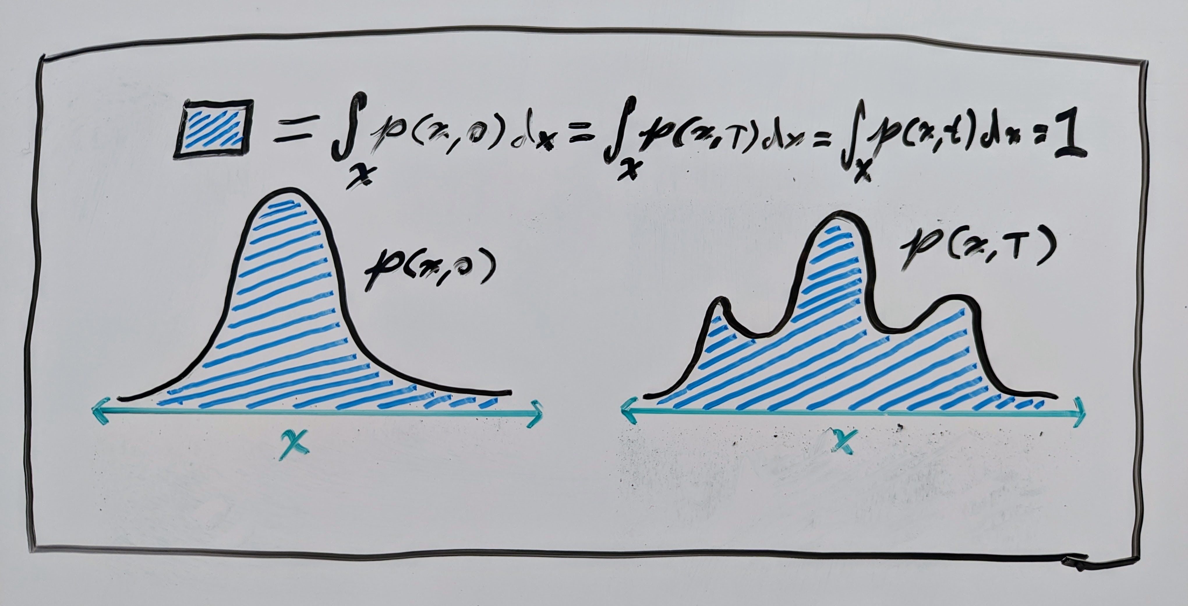
$$ \frac{\partial p(\mathbf{x}, t)}{\partial t} = -\nabla_\mathbf{x} \cdot \left(\mathbf{v}(\mathbf{x}, t) p(\mathbf{x}, t)\right) $$

where $p : \mathbb{R}^n \times \mathbb{R}_{\geq0} \to \mathbb{R}_{\geq 0}$ is a time-dependent “density” and $\nabla_\mathbf{x} \cdot$ is the divergence operator. This equation essentially says that the total mass of the system does not change over time. In our case, this “mass” is just the total probability of the space, which is $\int p(\mathbf{x}, t) \mathrm{d}\mathbf{x} = 1$ for probability density functions (PDFs). See another fantastic art piece below for an illustration.

**Figure**: The continuity equation preserves the total mass of the PDF!

So, if the VF and PDF $(\mathbf{v}, p)$ satisfy the continuity equation, then we can say that $\mathbf{v}$ generates $p$. This also means that the well-known change-of-variables equation is satisfied (see Chapter 1 of Villani’s book on optimal transport for details):

$$ p(\mathbf{x}, t) = p(\mathbf{\phi}^{-1}(\mathbf{x}, t), 0) \det \left(\nabla_\mathbf{x} \mathbf{\phi}^{-1}(\mathbf{x}, t) \right) $$

where $\mathbf{\phi}: \mathbb{R}^n \times \mathbb{R}_{\geq 0} \to \mathbb{R}^n$ is a flow map (or integral curve) of $\mathbf{v}$ starting from $\mathbf{x}$, defining an ordinary differential equation (ODE)

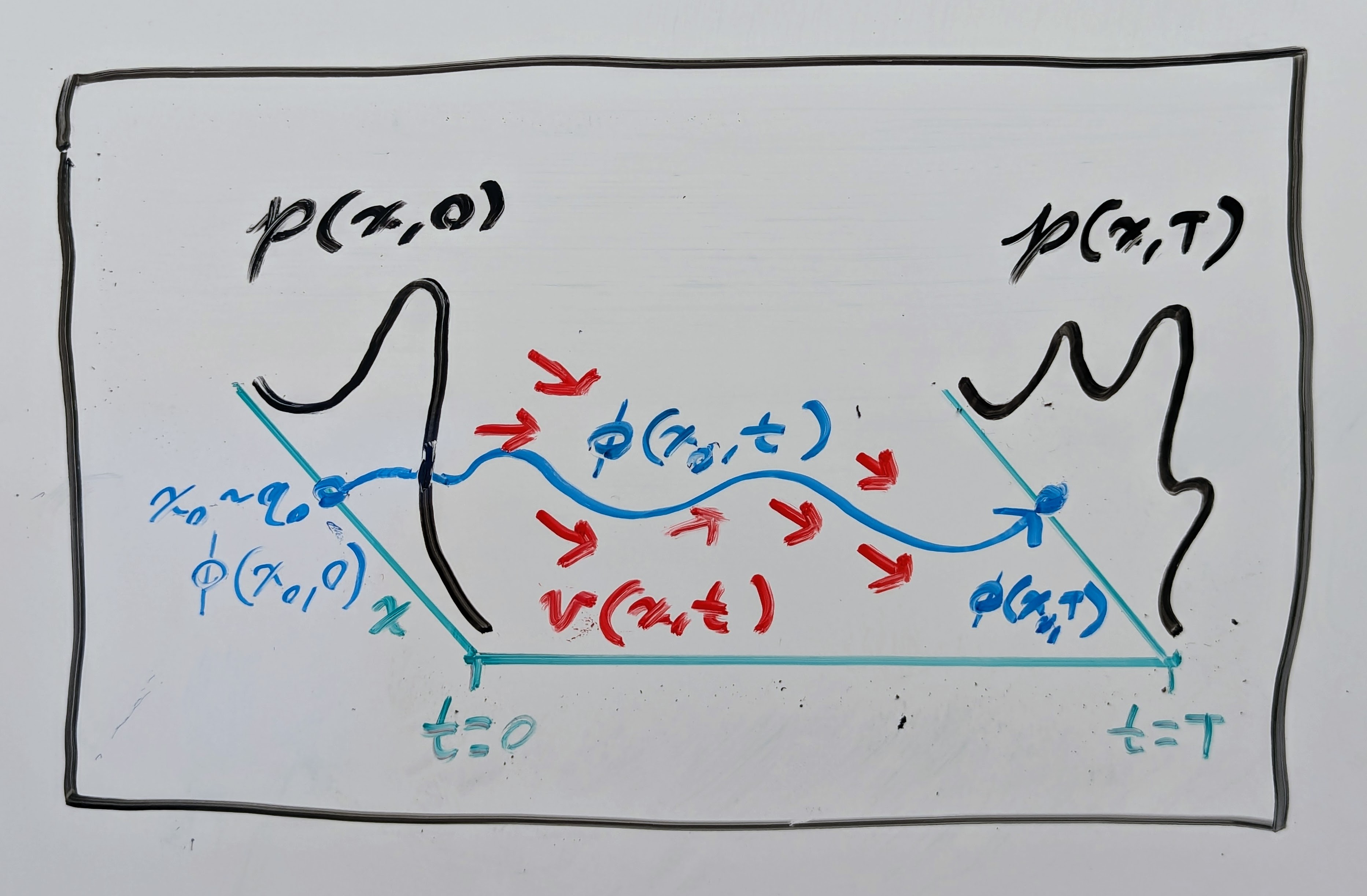
$$ \frac{\mathrm{d} \mathbf{\phi}(\mathbf{x}, t)}{\mathrm{d} t} = \mathbf{v}(\mathbf{\phi}(\mathbf{x}, t), t); $$

$\mathbf{\phi}^{-1}(\mathbf{x}, t)$ is its inverse with respect to $\mathbf{x}$; and $\nabla_\mathbf{x} \mathbf{\phi}^{-1}(\mathbf{x}, t)$ is the Jacobian matrix with respect to $\mathbf{x}$ of its inverse. Essentially, this is just a theoretical justification saying that we can sample $\mathbf{x}_0 \sim q_0$ and then compute $\mathbf{x}_1 = \mathbf{\phi}(\mathbf{x}_0, T)$ through numerical integration of $\mathbf{v}$ starting from $\mathbf{x}_0$ to get a sample from the complex distribution $\mathbf{x}_1 \sim q_1$. See another drawing below!

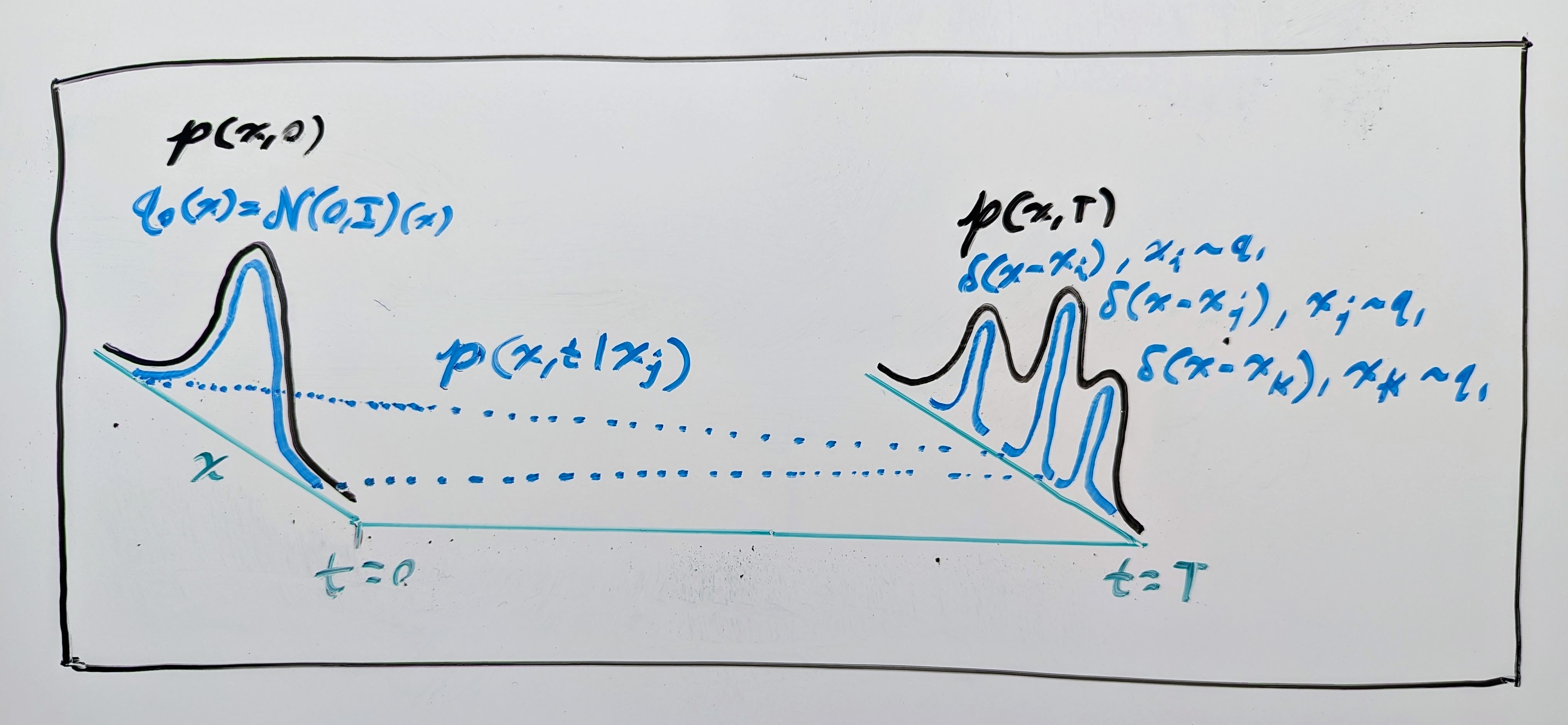
**Figure**: A flow map $\mathbf{\phi}(\mathbf{x}, t)$ from $t = 0$ to $t = T$.

Okay, but there is one big problem here: how do we actually learn a model of such a vector field $\mathbf{v}$ if we only have samples from the simple and complex PDFs, $q_0$ and $q_1$? Well, the flow matching (FM) authors proposed learning from intermediate samples of a conditional PDF $p(\mathbf{x}, t \mid \mathbf{x}_1)$ that converges to a concentrated PDF (i.e. a Dirac delta distribution $\delta$) around each data sample $\mathbf{x}_1 \sim q_1$ such that it locally emulates the desired PDF (see drawing below). I.e. we design $p(\mathbf{x}, t \mid \mathbf{x}_1)$ such that, for some time $T \in \mathbb{R}_{\geq 0}$, we have:

$$ \lim_{t \to T} p(\mathbf{x}, t \mid \mathbf{x}_1) \approx \delta(\mathbf{x} - \mathbf{x}_1). $$

**Figure**: $q_0$ being transported to $\delta(\mathbf{x} - \mathbf{x}_1)$ for each $\mathbf{x}_1 \sim q_1$.

Just like before, the conditional PDF $p(\mathbf{x}, t \mid \mathbf{x}_1)$ also has a vector field $\mathbf{v}(\mathbf{x}, t \mid \mathbf{x}_1)$ that generates it, so it also has a continuity equation:

$$ \frac{\partial p(\mathbf{x}, t \mid \mathbf{x}_1)}{\partial t} = -\nabla_\mathbf{x} \cdot \left(\mathbf{v}(\mathbf{x}, t \mid \mathbf{x}_1) p(\mathbf{x}, t \mid \mathbf{x}_1)\right). $$

The FM authors then make the assumption that the desired PDF can be constructed by a “mixture” of the conditional PDFs:

$$ p(\mathbf{x}, t) = \int p(\mathbf{x} \mid \mathbf{x}_1) q_1(\mathbf{x}_1) \mathrm{d} \mathbf{x}_1, $$

where the desired PDF $p(\mathbf{x}, t)$ can be interpreted as the “marginal PDF”. With this assumption, they then identify a marginal VF by using both the marginal and conditional continuity equations:

$$ \begin{aligned} \frac{\partial p(\mathbf{x}, t)}{\partial t} &= \frac{\partial}{\partial t} \int p(\mathbf{x} \mid \mathbf{x}_1) q_1(\mathbf{x}_1) \mathrm{d} \mathbf{x}_1 \\ &= \int \frac{\partial p(\mathbf{x} \mid \mathbf{x}_1)}{\partial t} q_1(\mathbf{x}_1) \mathrm{d} \mathbf{x}_1 \\ &= \int -\nabla_\mathbf{x} \cdot \left(\mathbf{v}(\mathbf{x}, t \mid \mathbf{x}_1) p(\mathbf{x}, t \mid \mathbf{x}_1)\right) q_1(\mathbf{x}_1) \mathrm{d} \mathbf{x}_1 \\ &= -\nabla_\mathbf{x} \cdot \left(\int \mathbf{v}(\mathbf{x}, t \mid \mathbf{x}_1) p(\mathbf{x}, t \mid \mathbf{x}_1) q_1(\mathbf{x}_1) \mathrm{d} \mathbf{x}_1\right) \\ &= -\nabla_\mathbf{x} \cdot \left(\mathbf{v}(\mathbf{x}, t) p(\mathbf{x}, t)\right) \\ \\ \implies \mathbf{v}(\mathbf{x}, t) &= \frac{1}{p(\mathbf{x}, t)} \int \mathbf{v}(\mathbf{x}, t \mid \mathbf{x}_1) p(\mathbf{x}, t \mid \mathbf{x}_1) q_1(\mathbf{x}_1) \mathrm{d} \mathbf{x}_1. \end{aligned} $$

Based on the marginal VF $\mathbf{v}(\mathbf{x}, t)$, the FM authors showed that we can train an NN VF $\mathbf{v}_\theta$ to match the conditional VFs:

$$ \begin{aligned} L_\text{FM}(\theta) &= \underset{\substack{t \sim \mathcal{U}[0, T] \\ \mathbf{x} \sim p(\mathbf{x}, t)}}{\mathbb{E}} \lVert \mathbf{v}_\theta(\mathbf{x}, t) - \mathbf{v}(\mathbf{x}, t) \rVert^2\\ L_\text{CFM}(\theta) &= \underset{\substack{t \sim \mathcal{U}[0, T] \\ \mathbf{x}_1 \sim q_1(\mathbf{x}_1)\\ \mathbf{x} \sim p(\mathbf{x}, t \mid \mathbf{x}_1)}}{\mathbb{E}} \lVert \mathbf{v}_\theta(\mathbf{x}, t) - \mathbf{v}(\mathbf{x}, t \mid \mathbf{x}_1) \rVert^2 \\ \nabla_\theta L_\text{FM}(\theta) &= \nabla_\theta L_\text{CFM}(\theta) \end{aligned} $$

where $L_\text{FM}$ matches the NN VF to the unknown desired VF $\mathbf{v}(\mathbf{x}, t)$ (what we originally wanted to do) and $L_\text{CFM}$ matches the NN VF to the conditional VFs $\mathbf{v}(\mathbf{x}, t \mid \mathbf{x}_1)$. Since their gradients are equal, minimizing them should, in theory, result in the same NN VF $\mathbf{v}_\theta(\mathbf{x}, t)$. Check Theorem 1 and Theorem 2 of the FM paper to see the original proof of the marginal VF and CFM loss equivalence.

Here’s where things get interesting. Similar to the marginal PDF $p(\mathbf{x}, t)$, the marginal VF $\mathbf{v}(\mathbf{x}, t)$ is a mixture of conditional VFs $\mathbf{v}(\mathbf{x}, t \mid \mathbf{x}_1)$. What does this “mixture” actually mean? In the case of the marginal PDF $p(\mathbf{x}, t)$, this mixture is just the marginalization of the conditional PDFs $p(\mathbf{x}, t \mid \mathbf{x}_1)$ over all samples of the complex distribution $\mathbf{x}_1 \sim q_1$. But, for the marginal VF $\mathbf{v}(\mathbf{x}, t)$, it is a bit less clear, but qualitatively it must be some weighted combination of the conditional VFs $\mathbf{v}(\mathbf{x}, t \mid \mathbf{x}_1)$. Let’s take a look at the terms in the marginal VF $\mathbf{v}(\mathbf{x}, t)$ expression other than the conditional VF:

$$ \frac{1}{p(\mathbf{x}, t)} \int p(\mathbf{x}, t \mid \mathbf{x}_1) q(\mathbf{x}_1) \mathrm{d}\mathbf{x}_1 = \frac{p(\mathbf{x}, t)}{p(\mathbf{x}, t)} = 1. $$

This means that, in fact, the marginal VF is a convex combination of the conditional VFs, where the weights are all positive (PDFs are always positive) and sum to $1$. Since the marginal VF $\mathbf{v}(\mathbf{x}, t)$ admits a flow map $\mathbf{\phi}(\mathbf{x}, t)$, we then have something called a differential inclusion:

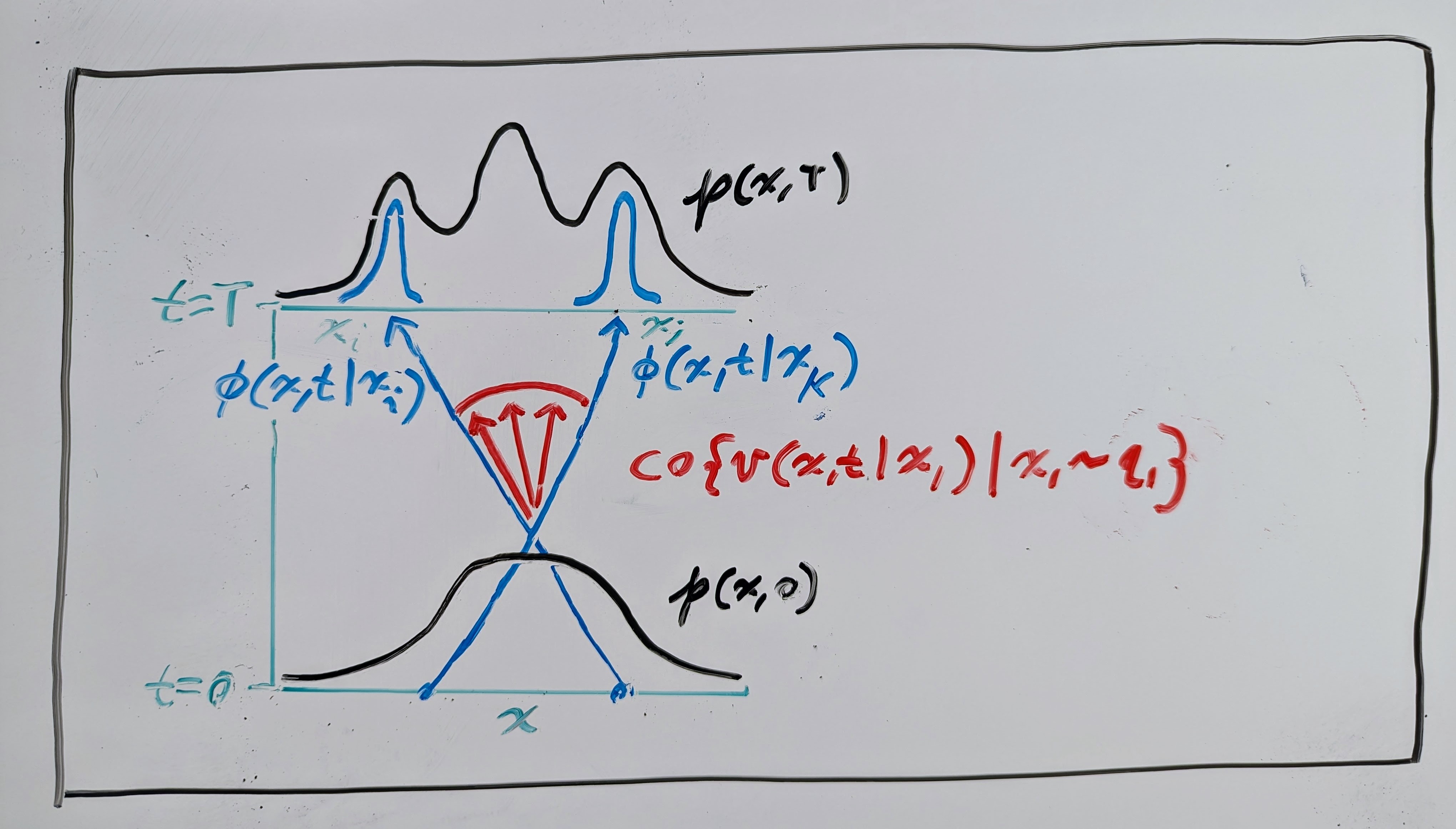
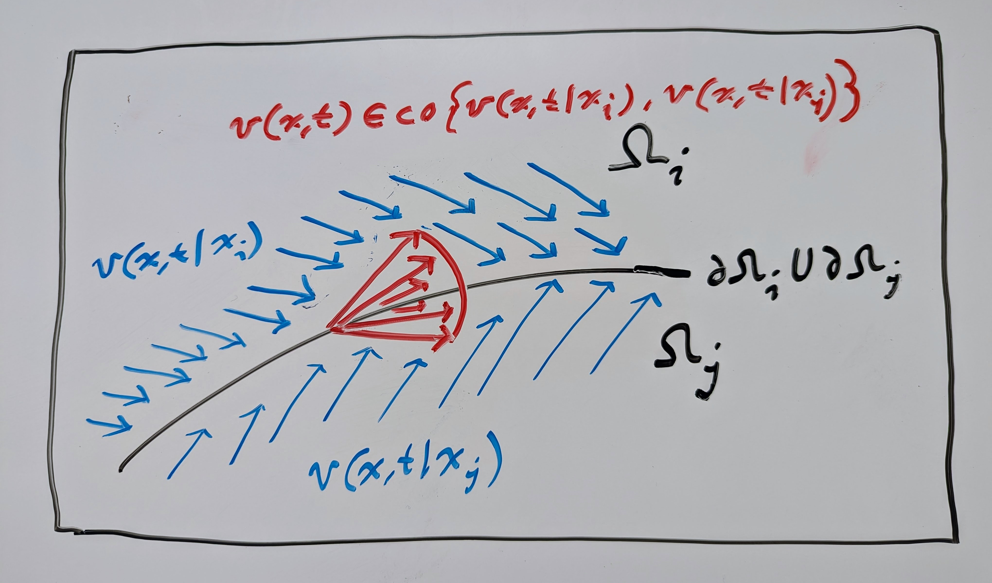
$$ \frac{\mathrm{d} \mathbf{\phi}(\mathbf{x}, t)}{\mathrm{d} t} \in \mathrm{co} \left\{\mathbf{v}(\mathbf{\phi}(\mathbf{x}, t), t \mid \mathbf{x}_1) \mid \mathbf{x}_1 \sim q_1 \right\}, $$

where $\mathrm{co}$ is the convex hull operator, which gives the set of all possible convex combinations. Take a look at the red vectors in the drawing below; the set of all positively weighted averages (convex combination) of these vectors is the convex hull.

**Figure**: The marginal VF lies in some convex combination of the conditional VFs (red).

Differential inclusions were introduced in the 1960s by Filippov (Филиппов) as a way to characterize solutions to ODEs with discontinuous VFs (see Filippov’s book on differential inclusions). They are an integral part of discontinuous dynamical systems (DDSs), where several VFs interface on a partitioned domain (see the drawing below). I recommend Cortes’ article on DDSs for a complete description.

DDSs with differential inclusions are commonplace in hybrid dynamical systems (HDSs), such as switched systems or behavior trees (BTs) (shameless plug to my PhD research). For a complete description, I recommend this article on HDSs by Goebel, Sanfelice, and Teel; and this article on switched systems by Liberzon.

Switched systems are of particular relevance to the marginal VF $\mathbf{v}(\mathbf{x}, t)$ discussed above. In switched systems, there is a “switching signal” $\sigma$ that indicates which VF to use (the conditional VFs $\mathbf{v}(\mathbf{x}, t \mid \mathbf{x}_1)$ in our case). This signal may be state-dependent $\sigma: \mathbb{R}^n \to \mathbb{N}$ or time-dependent $\sigma: \mathbb{R}_{\geq 0} \to \mathbb{N}$, where $\mathbb{N}$ (natural numbers) contains the index set of the individual VFs (or “subsystems”). If we adapt this to work with the conditional VFs above, the switching signal would map like $\sigma: \mathbb{R}^n \to \mathrm{supp}(q_1)$ for the state-dependent case and $\sigma: \mathbb{R}_{\geq 0} \to \mathrm{supp}(q_1)$ for the time-dependent case, where $\mathrm{supp}(q_1)$ is the support of the complex PDF (i.e. where there is non-zero probability).

If the switching signal is only state-dependent, then we end up with a DDS that looks like the picture below, where the conditional VFs $\mathbf{v}(\mathbf{x}, t \mid \mathbf{x}_1)$ are assigned to each partition of the domain, i.e.:

$$ \frac{\mathrm{d} \mathbf{\phi}(\mathbf{x}, t)}{\mathrm{d} t} = \mathbf{v}(\mathbf{\phi}(\mathbf{x}, t), t \mid \sigma(\mathbf{\phi}(\mathbf{x}, t))). $$

**Figure**: A DDS with two domains such that $\sigma(\mathbf{x}, t) = \mathbf{x}_i \in \mathrm{supp}(q_1)$ for all $\mathbf{x} \in \Omega_i \subset \mathbb{R}^n $ and $\sigma(\mathbf{x}, t) = \mathbf{x}_j \in \mathrm{supp}(q_1)$ for all $\mathbf{x} \in \Omega_j \subset \mathbb{R}^n $, where the domains partition the space, i.e. $\Omega_i \cap \Omega_j = \emptyset$ and $\Omega_i \cup \Omega_j = \mathbb{R}^n$. A Filippov solution will involve a convex combination of the VFs on the switching boundary $\partial \Omega_i \cup \partial \Omega_j$.

In the time-dependent case, the switching signal defines a schedule of switching times that determines which intervals of time to use a particular conditional VF, i.e.

$$ \frac{\mathrm{d} \mathbf{\phi}(\mathbf{x}, t)}{\mathrm{d} t} = \mathbf{v}(\mathbf{\phi}(\mathbf{x}, t), t \mid \sigma(t)). $$

Here the switching signal $\sigma(t)$ can be viewed as an open-loop control policy that we design or that we do not know (could come from external disturbances). A crucial problem in switched systems is determining whether the system will be stable to some desired state (i.e. converges to the state and stays there). In our case, we would want the flow map to be stable to samples of the complex distribution.

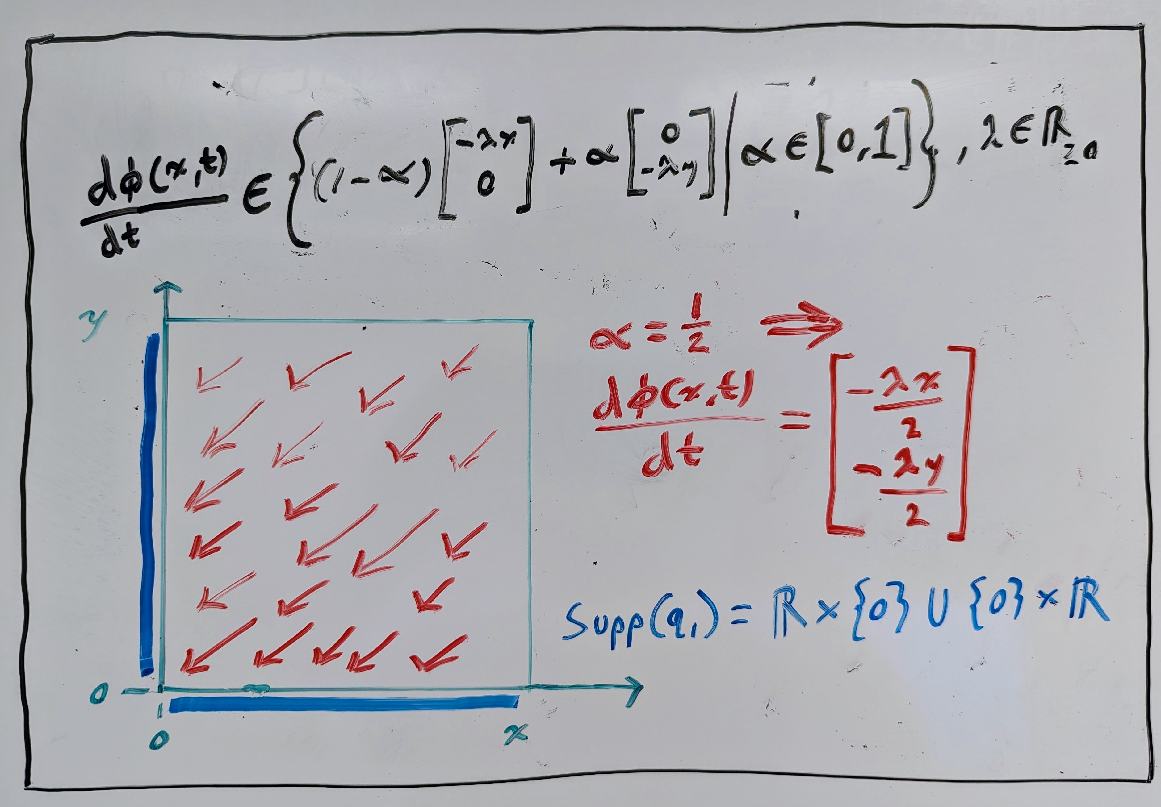
Now let’s assume that we do not know the switching signal. In this case, it suffices to show “stability under arbitrary switching” (see chapter 4 of Liberzon’s article on switched systems), which essentially shows the stability of the differential inclusion. If we can prove that all convex combinations of the conditional VFs $\mathbf{v}(\mathbf{x}, t \mid \mathbf{x}_1)$ are stable, then we can prove that the marginal VF $\mathbf{v}(\mathbf{x}, t)$ is stable. See the drawing below, where there is a convex combination of two 2D linear VFs. Every flow map $\mathbf{\phi}(\mathbf{x}, t)$ of every convex combination of these VFs will converge exponentially to the manifold in blue, which we can imagine as the support of the complex PDF $q_1$.

**Figure**: A convex combination of two 2D linear VFs is shown in red. All convex combinations will be stable to the manifold in blue. Imagine that this manifold is the support of the complex PDF. If $\alpha = 0$ the VF will point to the left, if $\alpha = 1$ the VF will point down.

Now, why would we care about stability in generative models? Well, of course we would want the flow maps $\mathbf{\phi}(\mathbf{x}, t)$ of the VF $\mathbf{v}(\mathbf{x}, t)$ to converge to samples of the complex distribution $\mathbf{x}_1 \sim q_1$ so that we generate the data we want. But, in some applications, it may also be desirable to have it so that the flow maps $\mathbf{\phi}(\mathbf{x}, t)$ stay stable to the samples $\mathbf{x}_1 \sim q_1$. For instance, in the context of structural biology, we may want to use a generative model to predict how a given ligand (e.g. serotonin) binds to a given receptor (e.g. the serotonin receptor). It is well-known in structural biology that molecular binding configurations represent minima of a “free energy landscape”. It is also well-known in control theory that energy can often be used as an effective Lyapunov function $V: \mathbb{R}^n \times \mathbb{R}_{\geq 0} \to \mathbb{R}_{\geq 0}$, which is just a scalar function that can be used to certify that the VF $\mathbf{v}(\mathbf{x}, t)$ is stable within some region $\mathcal{B} \subset \mathbb{R}^n$. To be a Lyapunov-like function on a region $\mathcal{B}$, we need to have the following for all $(\mathbf{x}, t) \in \mathcal{B} \times \mathbb{R}_{\geq 0}$:

$$ \mathcal{L}_\mathbf{v} V (\mathbf{x}, t) = \frac{\partial V(\mathbf{x}, t)}{\partial t} + \nabla_\mathbf{x}V(\mathbf{x}, t) \mathbf{v}(\mathbf{x}, t) \leq 0, $$

where $\mathcal{L}_\mathbf{v}$ is known as the Lie derivative operator. If this condition is satisfied, then it means that $V(\mathbf{x}, t)$ is always decreasing if $\mathbf{x} \in \mathcal{B}$, and the flow map $\mathbf{\phi}(\mathbf{x}, t)$ will eventually converge to one of the minima of $V(\mathbf{x}, t)$:

\[\lim_{t \to \infty} \mathbf{\phi}(\mathbf{x}, t) \in \left\{\mathbf{x} \in \mathbb{R}^n \mid \mathcal{L}_\mathbf{v} V(\mathbf{x}, t) = 0 \right\}.\]

Now how do we enforce the condition $\mathcal{L}_\mathbf{v} V (\mathbf{x}, t) \leq 0$? Of course, if the marginal VF $\mathbf{v}(\mathbf{x}, t)$ just follows the negative gradient of this function, i.e. $\mathbf{v}(\mathbf{x}, t) = -\nabla_\mathbf{x} V(\mathbf{x}, t)$ (a gradient flow), then the second term in $\mathcal{L}_\mathbf{v} V (\mathbf{x}, t)$ will be non-positive. The hard bit is ensuring that the first term in $\mathcal{L}_\mathbf{v} V (\mathbf{x}, t)$ with the time derivative is non-positive, which could normally be achieved by making the marginal VF $\mathbf{v}(\mathbf{x}, t)$ time-independent.

But, even if we make the conditional VFs time-independent, $\mathbf{v}(\mathbf{x} \mid \mathbf{x}_1)$, the marginal VF will still be time-dependent, $\mathbf{v}(\mathbf{x}, t)$, due to its dependence on the conditional $p(\mathbf{x}, t \mid \mathbf{x}_1)$ and marginal PDF $p(\mathbf{x}, t)$:

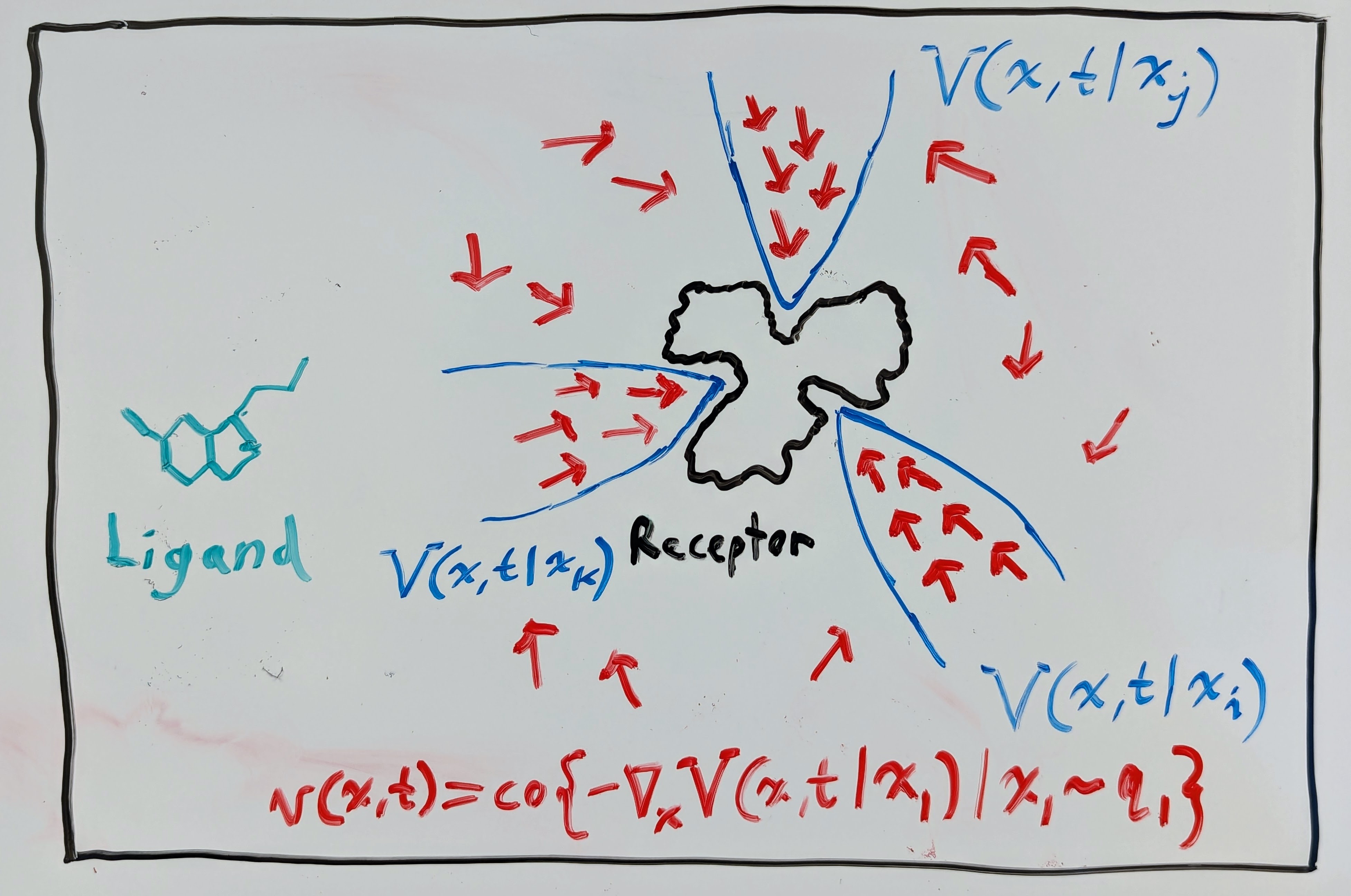
$$ \mathbf{v}(\mathbf{x}, t) = \frac{1}{p(\mathbf{x}, t)} \int \mathbf{v}(\mathbf{x} \mid \mathbf{x}_1) p(\mathbf{x}, t \mid \mathbf{x}_1) q_1(\mathbf{x}_1) \mathrm{d} \mathbf{x}_1. $$

Assume for the moment, though, that there does exist a Lyapunov-like free-energy function $V(\mathbf{x}, t)$ satisfying the Lyapunov condition $\mathcal{L}_\mathbf{v} V (\mathbf{x}, t) \leq 0$. Then, in the context of ligand-receptor binding, we could have something like in the drawing below, where the marginal VF $\mathbf{v}(\mathbf{x}, t)$ follows the negative gradient of a mixture of Lyapunov functions.

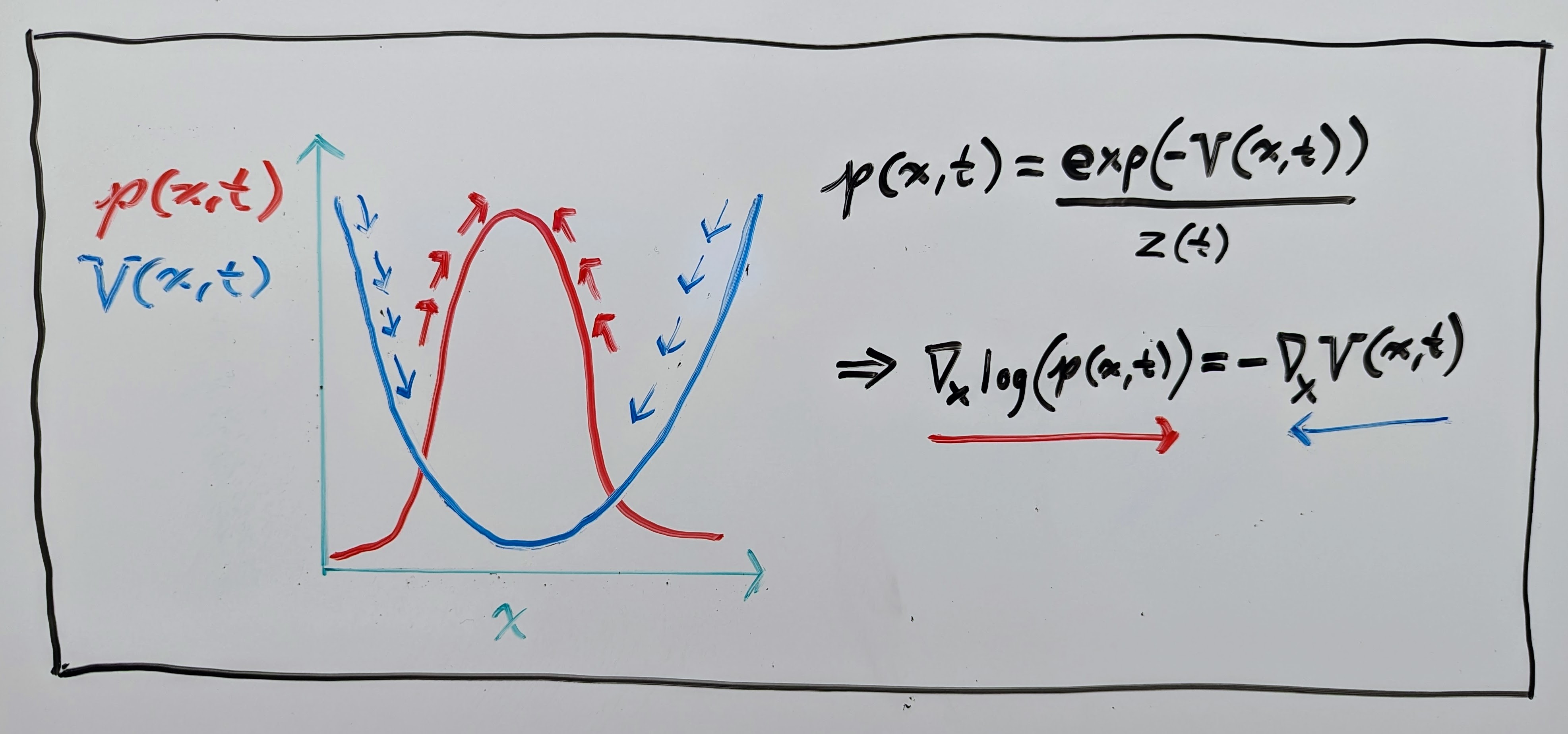
**Figure**: Energy descent in the context of ligand-receptor binding.

This interpretation is useful, as it is often assumed in structural biology that data follows a Boltzmann-like distribution:

$$ p(\mathbf{x}, t) = \frac{\exp(-V(\mathbf{x}, t))}{z(t)}, $$

where $z(t)$ is just a normalizing constant ensuring that the PDF integrates to $1$. If this is true, and our flow maps $\mathbf{\phi}(\mathbf{x}, t)$ are following the negative gradient of the energy function $V(\mathbf{x}, t)$, then it is easy to see that they also follow the gradient of the log probability $\log(p(\mathbf{x}, t))$ (shown in the drawing below):

$$ \nabla_\mathbf{x} \log \left(p(\mathbf{x}, t) \right) = -\nabla_\mathbf{x} V(\mathbf{x}, t). $$

**Figure**: The correspondence between energy descent and log probability ascent.

Now, how could this use of energy\Lyapunov-like functions be useful in a FM generative model that is used for generating physically stable samples? Let’s explain with the drug binding example.

It is well-known that ligands can bind to receptors in different ways. E.g., in the context of drugs, there are orthosteric and allosteric sites where drugs can bind. Orthosteric sites are where endogenous drugs (agonists) bind; e.g. serotonin is the endogenous agonist of the serotonin receptor. Allosteric sites are sites other than the orthosteric site, which are of increasing interest because they allow for specific allosteric modulation since they are less “conserved” than orthosteric sites. Simply put, orthosteric binding sites can look similar across several receptors (more conserved), while allosteric binding sites are more distinct (less conserved), meaning that an allosteric-modulation drug should have less affinity to other receptors (fewer side effects).

In general, there is an abundance of data on orthosteric binding compared to allosteric binding. So, if we consider training a FM generative model with a binding dataset (e.g. PDBBind), it is more likely than not that the learned model will be biased towards orthosteric binding sites. It is well-known in machine learning that inductive biases can help learning performance when there is a lack of data. So energy and Lyapunov stability (inductive biases) may be a good ingredients to “bake” into generative models tasked to generate physically stable data.

Unfortunately, actually implementing the stability principle discussed before still requires us to have the time-derivative of the energy/Lyapunov-like function be non-positive, i.e. $\frac{\partial V(\mathbf{x}, t)}{\partial t}$, which can be difficult in practice, because time is unbounded, i.e. $t \in \mathbb{R}_{\geq}$, and FM models are trained between $t=0$ and $t=1=T$ (because time is simply an interpolation parameter between $q_0$ and $q_1$).

Luckily, in our new paper, Stable Autonomous Flow Matching, we show how to remove time from the FM framework and learn a time-independent VF that transports samples from a simple distribution $q_0$ to a complex distribution $q_1$ with the stability principles discussed above!

We will explain these results in a future blog post. If you would like to cite this blog post, please use the following BibTeX entry.

@article{sprague2024stable,
  title={Stable Autonomous Flow Matching},
  author={Sprague, Christopher Iliffe and Elofsson, Arne and Azizpour, Hossein},
  journal={arXiv preprint arXiv:2402.05774},
  year={2024}
}